The Nestimate Compatibility Map

Mohammed Saqr

University of Eastern Finland

Sonsoles López-Pernas

University of Eastern Finland

Manuel J. Gómez

University of Murcia

One object, two packages

A ts_tna() model is not exported to Nestimate; it is a Nestimate object. This vignette maps what that buys, verb by verb: which parts of Nestimate’s analysis surface accept a tsn transition model directly, what question each verb answers, what each result draws, and which parts do not apply and why. The companion vignette vignette("nestimate-workflow", package = "tsn") runs a single analysis end to end; this one is the reference you consult when deciding which verb to reach for.

The running example is the model from that workflow: the 36 students of the srl daily panel, whose effort reports are cut at 40 and 70 on the 0-100 scale so the states mean something outside the sample.

library(tsn)
library(Nestimate)

data(srl)
students <- subset(srl, !is.na(effort))

effort_model <- ts_tna(
  students,
  value = "effort",
  id = "name",
  time = "day",
  discretization = "threshold",
  breaks = c(40, 70),
  labels = c("low", "moderate", "high")
)

class(effort_model)
#> [1] "ts_tna"          "netobject"       "cograph_network"

The class chain is the whole compatibility story. ts_tna is the tsn layer (it remembers the source series and discretization), netobject is what every Nestimate verb dispatches on, and cograph_network is what cograph::splot() renders. Nestimate’s own validator agrees:

validate_netobject(effort_model)

And because the object is a cograph_network, the model itself is one plot() away:

plot(effort_model, type = "network")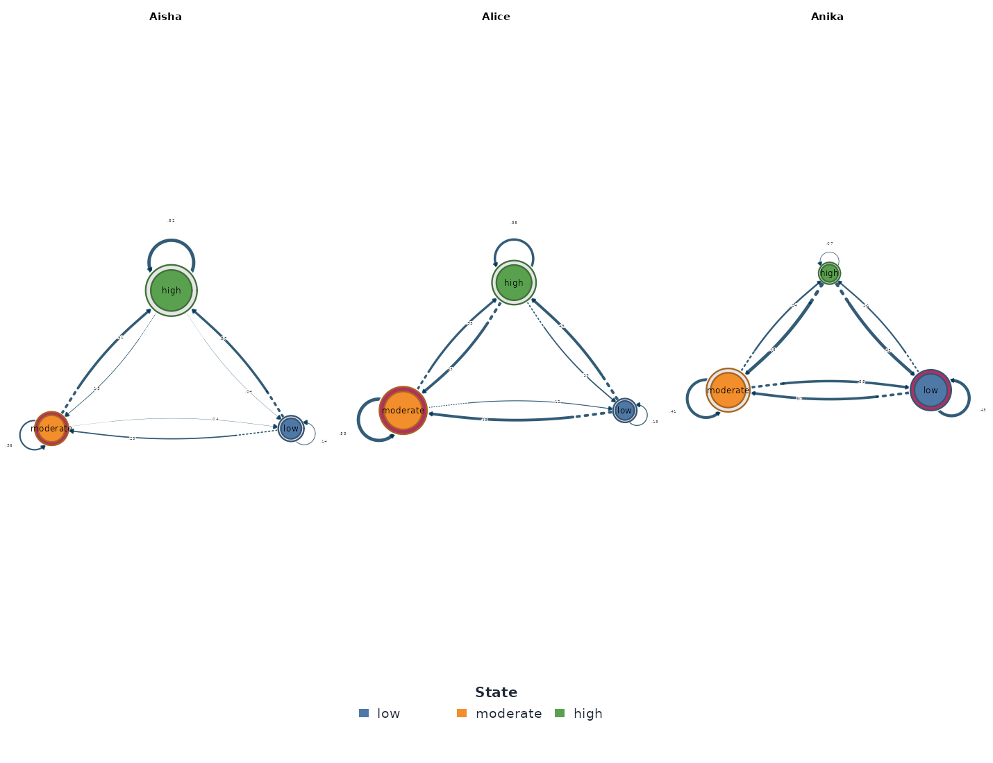

The strong diagonal is the first substantive fact: every state’s most likely successor is itself, high most strongly of all at 0.575.

Reading the model as data

Both packages provide accessors, and they answer slightly different questions. tsn’s as.data.frame() returns every state pair including self-transitions; as.matrix() returns the row-stochastic weight matrix.

head(as.data.frame(effort_model))
#>       from       to    weight
#> 1      low      low 0.4148311
#> 2 moderate      low 0.2184517
#> 3     high      low 0.1648021
#> 4      low moderate 0.3135095
#> 5 moderate moderate 0.4528102
#> 6     high moderate 0.2603270

Nestimate’s extractors return the same estimates in its own shapes:

extract_transition_matrix(effort_model)
#>                low  moderate      high
#> low      0.4148311 0.3135095 0.2716593
#> moderate 0.2184517 0.4528102 0.3287381
#> high     0.1648021 0.2603270 0.5748709
#> attr(,"class")
#> [1] "nest_transition_matrix" "matrix"                 "array"

extract_initial_probs(effort_model)
#>       low  moderate      high 
#> 0.1944444 0.3888889 0.4166667 
#> attr(,"class")
#> [1] "nest_initial_probs" "numeric"

extract_edges(effort_model)
#>       from       to    weight
#> 1 moderate     high 0.3287381
#> 2      low moderate 0.3135095
#> 3      low     high 0.2716593
#> 4     high moderate 0.2603270
#> 5 moderate      low 0.2184517
#> 6     high      low 0.1648021

One difference matters for transition networks: extract_edges() excludes self-transitions, returning the six between-state edges sorted by weight and omitting the diagonal. For this model the diagonal is where most of the probability lives (high → high is 0.575), so use as.data.frame() or extract_transition_matrix() whenever persistence is part of the question, and extract_edges() when only between-state movement is.

The initial-state probabilities say the panel starts engaged: 41.7% of students’ first recorded day is a high-effort day, 19.4% a low one.

Where the process spends its time

state_distribution() and state_frequencies() count observations per state, the marginal composition before any dynamics.

state_frequencies(effort_model)
#>      state count proportion
#> 1     high  2341     0.4174
#> 2 moderate  1900     0.3388
#> 3      low  1367     0.2438

High-effort days make up 41.7% of the panel and low-effort days 24.4%. Three displays draw the composition from different angles. The mosaic is the proportion bar:

mosaic_plot(effort_model)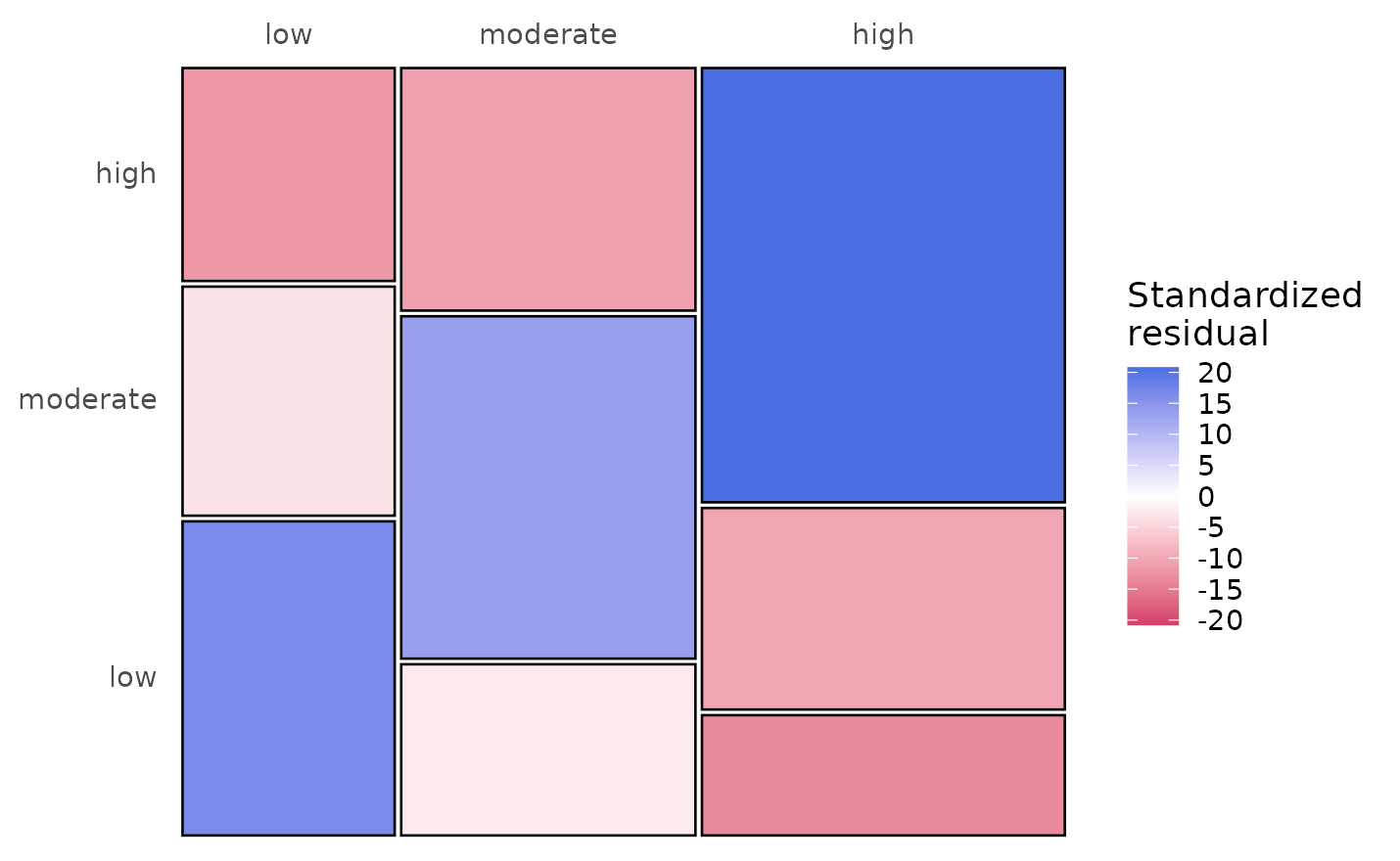

sequence_plot() is the sequence carpet, one row per student, one coloured cell per day:

sequence_plot(effort_model)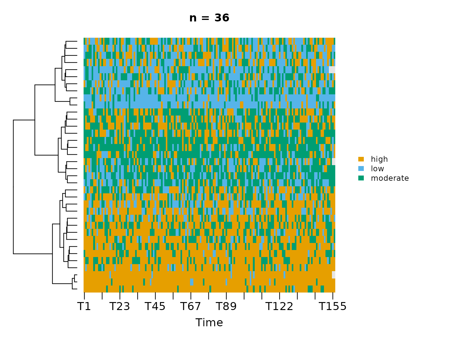

The streaks are persistence made visible: students hold a state for spells, not single days. distribution_plot() stacks the day-by-day state mix of the whole panel:

distribution_plot(effort_model)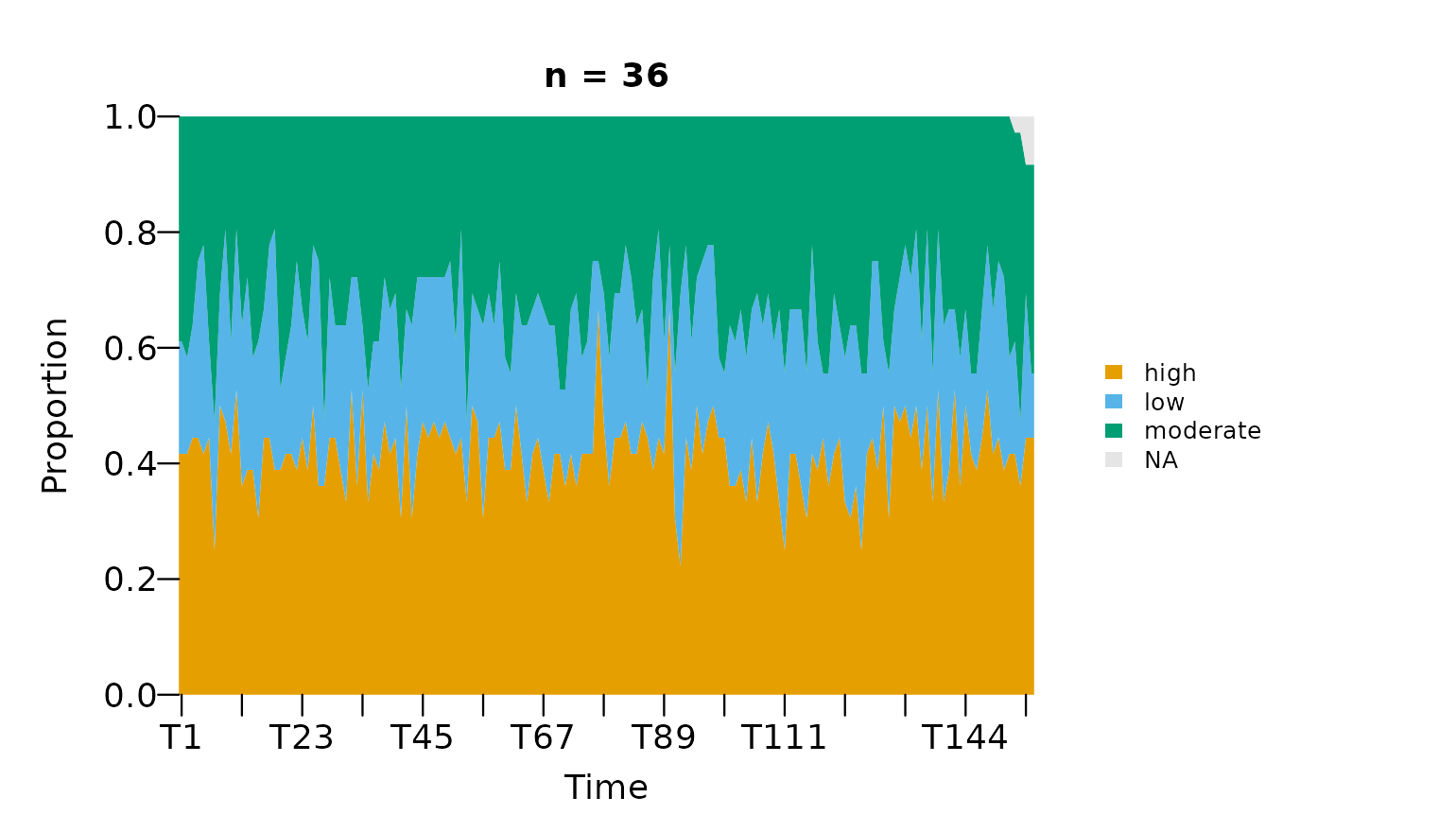

This is composition over course time, the view in which a first-to-second-half shift would appear, and the workflow vignette’s period comparison shows there is none. plot_state_frequencies() offers a fourth, marimekko-style variant of the same information.

Which states and edges carry the structure?

net_centrality() ranks states. Self-transitions are excluded by default, because for a transition network the diagonal would otherwise dominate every strength measure.

effort_centrality <- net_centrality(effort_model)
#> centralities computed excluding loops (diagonal). Pass `loops = TRUE` to include self-transitions.

effort_centrality
#>             state InStrength Betweenness Diffusion
#> low           low  0.3832538           0 1.0000000
#> moderate moderate  0.5738366           0 0.7292556
#> high         high  0.6003974           0 0.0000000

plot(effort_centrality)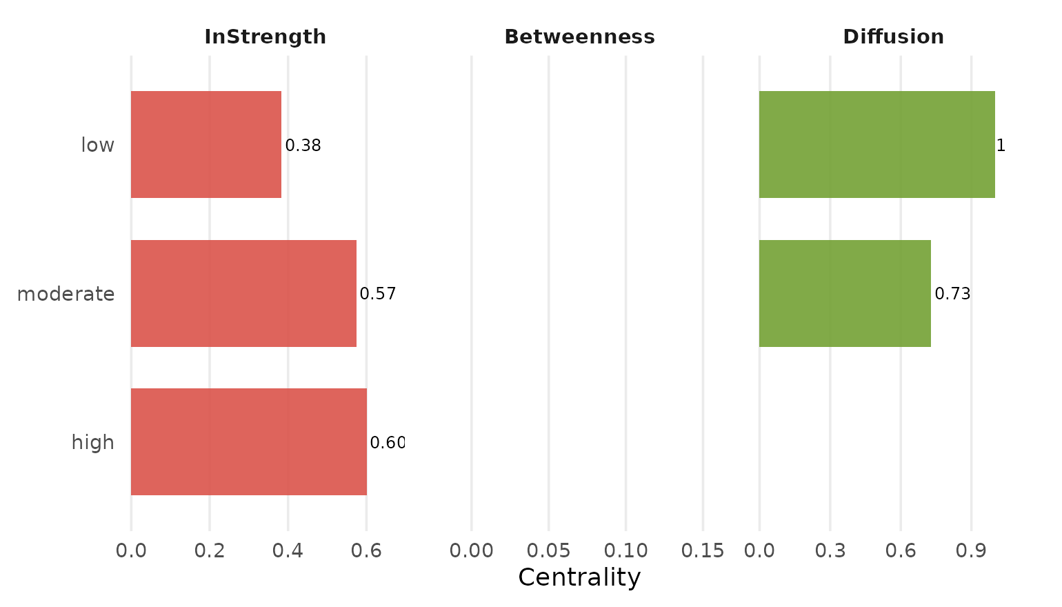

high and moderate receive similar between-state traffic (in-strengths of 0.60 and 0.57) while low receives markedly less (0.38); the betweenness column is uniformly zero because in a fully connected three-state network no state is an obligatory bridge.

net_edge_betweenness() asks the same question of edges:

effort_betweenness <- net_edge_betweenness(effort_model)

effort_betweenness
#> Network (method: edge_betweenness) [directed]
#>   Weights: [1.000, 1.000]  |  mean: 1.000
#> 
#>   Weight matrix:
#>            low moderate high
#>   low        0        1    1
#>   moderate   1        0    1
#>   high       1        1    0

plot(effort_betweenness)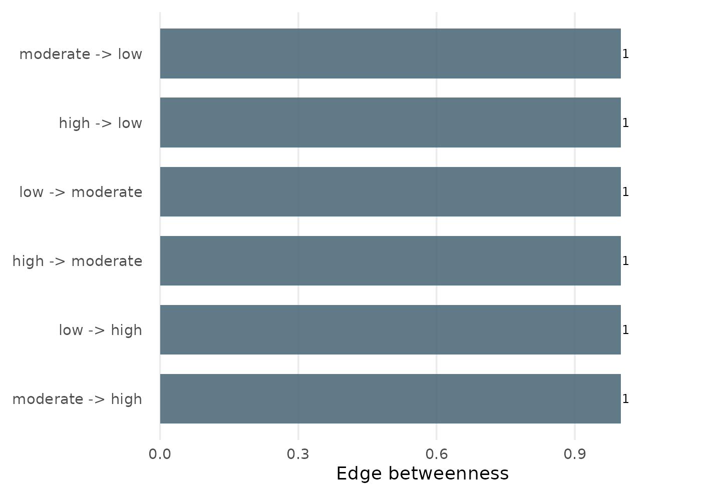

Every between-state edge carries the same load of 1: each lies on exactly one shortest path, and none is a privileged route. That uniformity is itself a description: movement between effort states does not funnel through any single corridor.

How the process moves

Mean first passage times

passage_time() converts the transition matrix into expected travel times between states (Kemeny & Snell, 1976).

effort_passage <- passage_time(effort_model)

effort_passage
#> Mean First Passage Times (3 states)
#> 
#>          low moderate high
#> low      4.1      3.4  3.4
#> moderate 5.1      3.0  3.2
#> high     5.5      3.7  2.4
#> 
#> Stationary distribution:
#>      low moderate     high 
#>   0.2440   0.3384   0.4176

plot(effort_passage)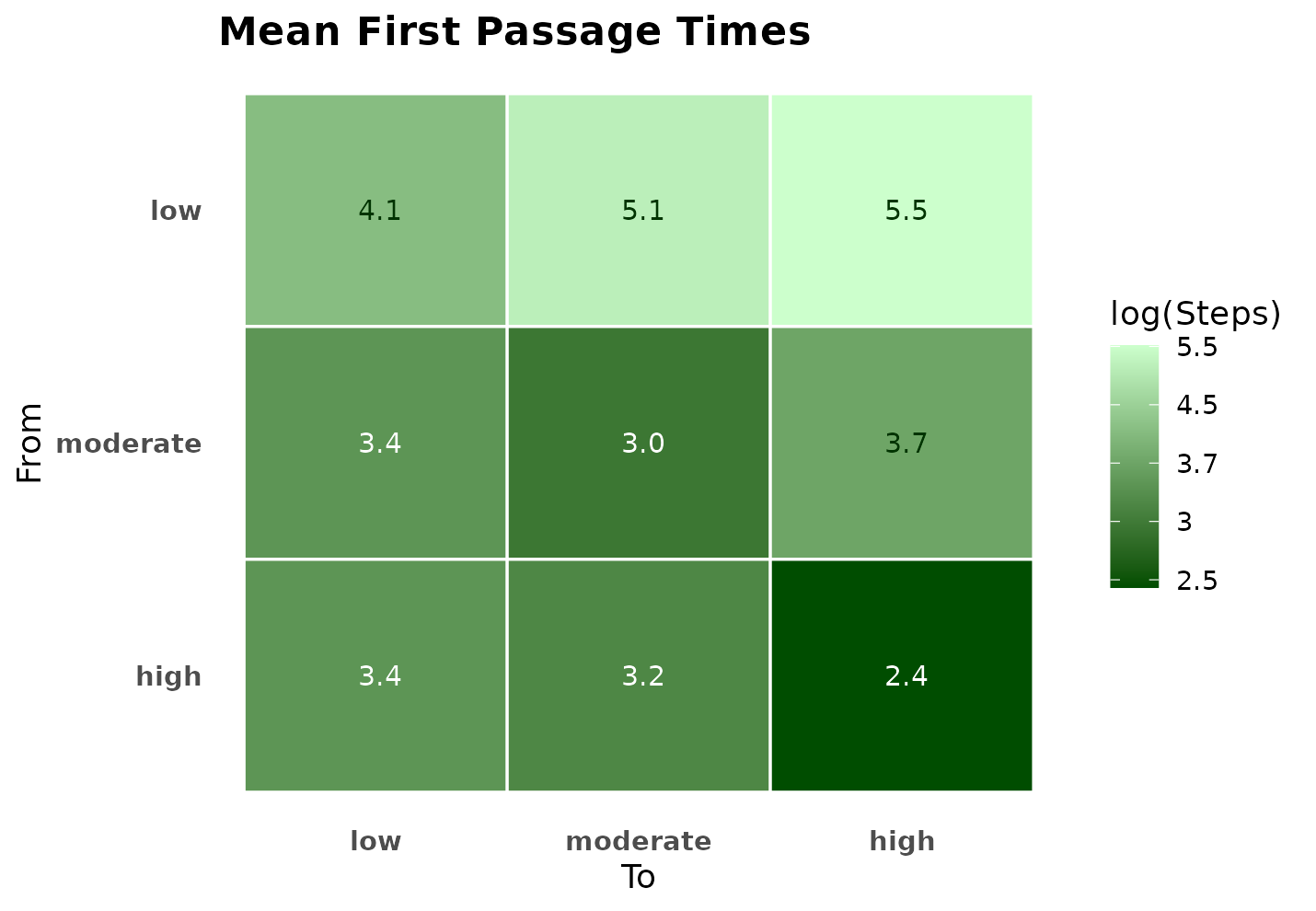

A moderate or high day is reached from anywhere within about two to four days on average; a low day takes four to five and a half. Low effort is the state this panel visits reluctantly, not a basin it falls into. The stationary distribution (24% low, 34% moderate, 42% high) is where the chain settles regardless of its start.

Persistence, return, and sojourn

markov_stability() summarizes each state’s dynamics in one row: the self-transition probability, the stationary share, the mean recurrence time, and the mean sojourn (how long a visit lasts once entered).

effort_spells <- markov_stability(effort_model)

effort_spells
#> Markov Stability Analysis
#> 
#>     state persistence stationary_prob return_time sojourn_time
#>       low      0.4148          0.2440        4.10         1.71
#>  moderate      0.4528          0.3384        2.95         1.83
#>      high      0.5749          0.4176        2.39         2.35
#>  avg_time_to_others avg_time_from_others
#>                3.42                 5.31
#>                4.16                 3.55
#>                4.58                 3.31

plot(effort_spells)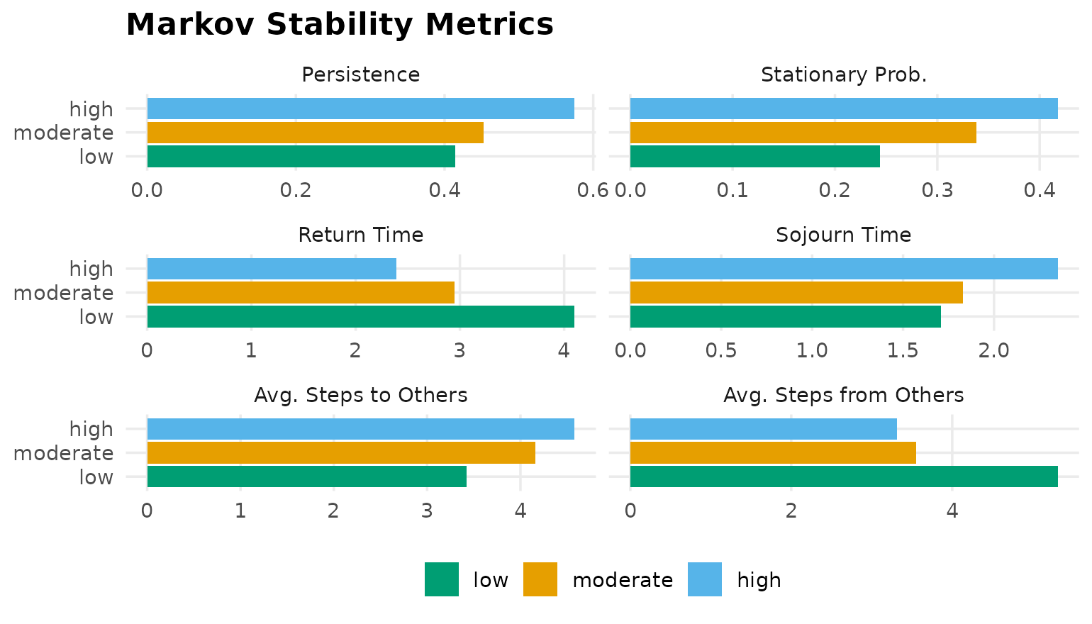

A high-effort spell lasts 2.4 days on average and recurs every 2.4; a low-effort spell lasts 1.7 days and recurs only every 4.1. Persistence and prevalence line up here, but they are logically distinct columns: a rare state can still be sticky.

Is the chain well-behaved?

chain_structure() reports the Markov-chain diagnostics that other verbs quietly assume: irreducibility (every state reachable from every other), aperiodicity, and reversibility.

summary(chain_structure(effort_model))
#> Chain structure summary  [3 states, 1 classes]
#>   irreducible: TRUE   aperiodic: TRUE   regular: TRUE   reversible: FALSE
#> 
#>     state classification period persistence return_probability sojourn_steps
#>       low      recurrent      1      0.4148                  1          1.71
#>  moderate      recurrent      1      0.4528                  1          1.83
#>      high      recurrent      1      0.5749                  1          2.35
#>  stationary_probability
#>                  0.2440
#>                  0.3384
#>                  0.4176

The chain is irreducible, aperiodic, and regular, so the stationary distribution above is well-defined and unique. It is not reversible: the forward process is statistically distinguishable from its time reversal, which is itself a substantive fact about self-regulation: the routes up the effort scale and the routes down are not mirror images.

How predictable is the process?

transition_entropy() gives the point estimate; entropy_bayes() adds a posterior credible interval by placing a Dirichlet prior on each row.

set.seed(2026)
effort_entropy <- entropy_bayes(effort_model)

effort_entropy
#> Bayesian Transition Entropy (3 states, bits; Dirichlet prior 0.5, 4000 draws)
#> 
#>   entropy_rate:       1.478 [1.462, 1.493]
#>    stationary_entropy: 1.551 [1.540, 1.561]
#>    redundancy:         0.073 [0.061, 0.086]
#> 
#> Edges: 9 observed; 9 credible (share of h(P) credibly > 1%).
#> Use summary() for the edge table, plot() for the posterior, and
#> $model for the pruned stable entropy network.

plot(effort_entropy)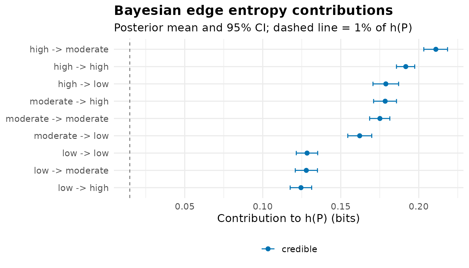

The entropy rate is 1.478 bits against a ceiling of log2(3) = 1.585, or 0.93 on the normalised scale, with a credible interval three hundredths wide: with 5,600 daily reports, the uncertainty about how unpredictable the process is, is itself small. The redundancy of 0.073 bits is the gap between the marginal entropy and the conditional one: knowing today’s effort removes under 5% of tomorrow’s uncertainty. Daily effort is mostly noise around a weak first-order signal, and every edge below should be read with that in mind.

entropy_network() maps the same quantity onto the edges, each entry an edge’s contribution to the row’s unpredictability, and returns a network of the same class, so it can be plotted or pruned like any other:

entropy_network(effort_model)
#> Network (method: entropy) [directed]
#>   Weights: [0.125, 0.211]  |  mean: 0.164
#> 
#>   Weight matrix:
#>              low moderate  high
#>   low      0.128    0.128 0.125
#>   moderate 0.162    0.175 0.179
#>   high     0.179    0.211 0.192 
#> 
#>   Initial probabilities:
#>   high          0.417  ████████████████████████████████████████
#>   moderate      0.389  █████████████████████████████████████
#>   low           0.194  ███████████████████

Does history beyond one step matter?

The model assumes the next state depends only on the current one. markov_order_test() (Anderson & Goodman, 1957) tests that assumption.

set.seed(2026)
effort_order <- markov_order_test(effort_model)

effort_order
#> Markov Order Test  [within-w permutation, n_perm = 500, alpha = 0.050]
#>   36 sequences / 5608 observations / 3 states
#> 
#>   Selected order  BIC: 2   AIC: 3   permutation-LRT: 3
#> 
#>  order   loglik      AIC      BIC df     g2 p_permutation  p_asymptotic
#>      0 -6031.21 12066.41 12079.67 NA     NA            NA            NA
#>      1 -5750.23 11516.45 11569.51  4 561.95   0.001996008 2.653668e-120
#>      2 -5606.12 11264.24 11436.67 12 288.17   0.001996008  1.422835e-54
#>      3 -5494.72 11149.43 11679.99 36 222.75   0.001996008  8.841816e-29
#>  significant
#>           NA
#>         TRUE
#>         TRUE
#>         TRUE

plot(effort_order)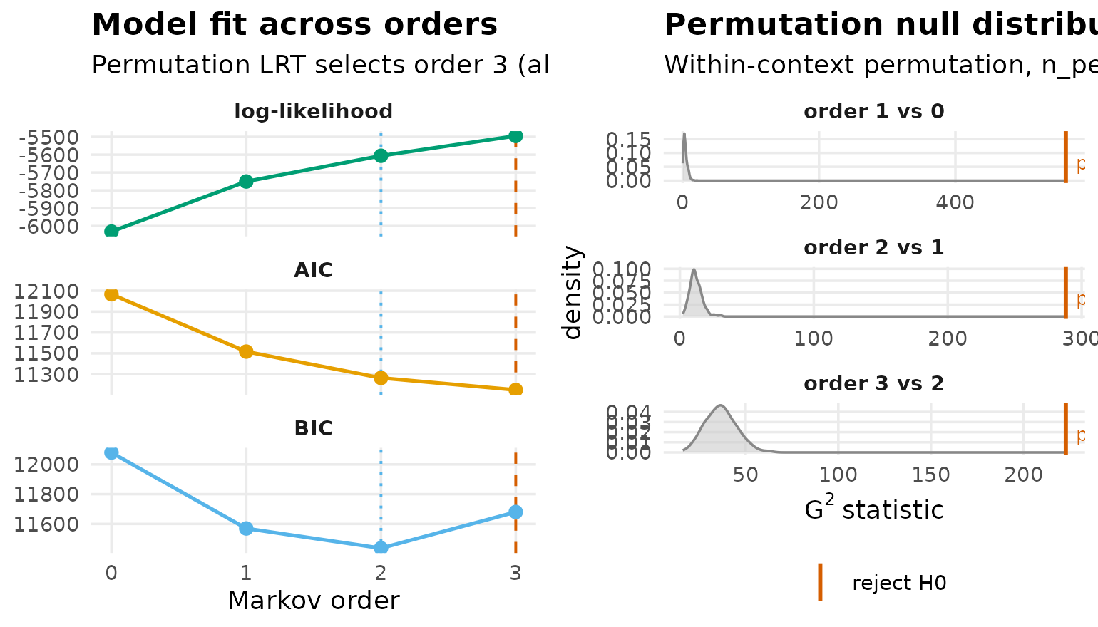

AIC and the permutation LRT select order 3 and BIC selects order 2: yesterday carries information about tomorrow beyond today. path_dependence() says how much:

effort_history <- path_dependence(effort_model)

effort_history
#> Path Dependence (order 2 vs order 1, bits)
#> 
#> Contexts: 9 (min_count = 5).  Modal-prediction flips: 2.
#> Chain-level KL_weighted      = 0.038 bits
#> Chain-level H_drop_weighted  = 0.037 bits
#> 
#> Top 9 contexts by KL:
#>               context    n H_order1 H_orderk H_drop    KL   top_o1   top_ok
#>           low -> high  366    1.393    1.570 -0.177 0.114     high     high
#>       low -> moderate  424    1.525    1.572 -0.047 0.050 moderate moderate
#>      moderate -> high  617    1.393    1.505 -0.112 0.048     high     high
#>      high -> moderate  599    1.525    1.478  0.046 0.037 moderate     high
#>          high -> high 1326    1.393    1.204  0.189 0.035     high     high
#>            low -> low  562    1.562    1.473  0.089 0.034      low      low
#>           high -> low  381    1.562    1.581 -0.019 0.032      low     high
#>  moderate -> moderate  849    1.525    1.471  0.054 0.014 moderate moderate
#>       moderate -> low  412    1.562    1.580 -0.018 0.011      low      low
#>  flips
#>  FALSE
#>  FALSE
#>  FALSE
#>   TRUE
#>  FALSE
#>  FALSE
#>   TRUE
#>  FALSE
#>  FALSE

plot(effort_history)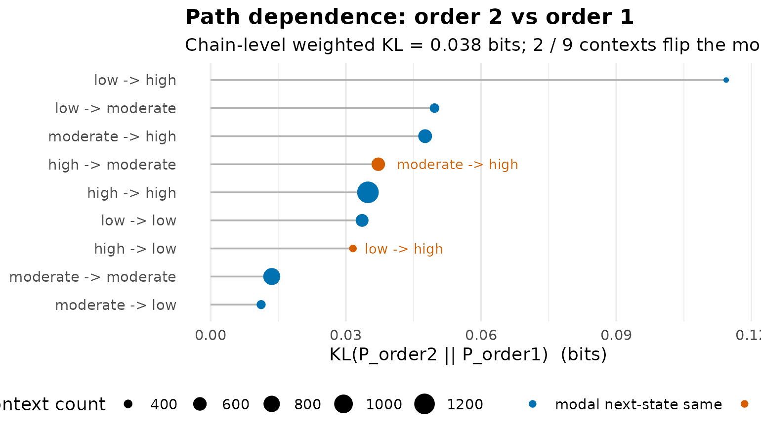

The weighted divergence is 0.038 bits: history shifts the next-step distribution by a few hundredths of a bit and flips the modal prediction in only two of nine contexts. This is the pair of numbers that reconciles a decisively significant order test with the continued use of a first-order model: detectable is not the same as large. The first-order network remains a fair one-step summary; it is not the full process.

path_counts() is the raw material, every observed two-step path with its count:

path_counts(effort_model)
#>                   path count proportion
#> 1         high -> high  1336     0.2398
#> 2 moderate -> moderate   854     0.1533
#> 3     moderate -> high   620     0.1113
#> 4     high -> moderate   605     0.1086
#> 5           low -> low   565     0.1014
#> 6      low -> moderate   427     0.0766
#> 7      moderate -> low   412     0.0739
#> 8          high -> low   383     0.0687
#> 9          low -> high   370     0.0664

high → high alone is 24.0% of all transitions. And when the order test demands more than one step, build_hon() estimates a higher-order network under its own per-node promotion rule:

hon <- build_hon(effort_model, max_order = 2)

pathways(hon)
#> character(0)

HON promotes no node here, because no single context shifts the next-step distribution enough to justify splitting a state, which is why pathways() comes back empty. Two criteria disagreeing is a result, not a bug: the likelihood test sees aggregate improvement, HON asks a stricter per-node question. Report both.

Simplifying the model

net_prune() removes weak edges and returns the same class; net_pruning_details() is the audit trail; net_deprune() undoes it.

pruned <- net_prune(effort_model, method = "threshold", threshold = 0.3)

net_pruning_details(pruned)
#> Pruning details
#>   Method:  user-specified threshold (0.3)
#>   Removed: 4 edges
#>   Retained: 5 edges
#> 
#>      from       to    weight
#>  moderate      low 0.2184517
#>      high      low 0.1648021
#>      high moderate 0.2603270
#>       low     high 0.2716593

Four edges fall, and they are a coherent four: every descending route (moderate → low, high → low, high → moderate) plus the direct low → high leap. What survives is the ascending ladder and the persistence loops. Because pruning is recorded rather than destructive, the original model is one call away:

net_deprune(pruned)
#> Transition Network (relative probabilities) [directed]
#>   Weights: [0.165, 0.575]  |  mean: 0.333
#> 
#>   Weight matrix:
#>              low moderate  high
#>   low      0.415    0.314 0.272
#>   moderate 0.218    0.453 0.329
#>   high     0.165    0.260 0.575 
#> 
#>   Initial probabilities:
#>   high          0.417  ████████████████████████████████████████
#>   moderate      0.389  █████████████████████████████████████
#>   low           0.194  ███████████████████

How sure are we about the estimates?

Nestimate offers several answers resting on different machinery: sequence resampling, node resampling, case dropping, sample splitting, and a posterior.

Sequence bootstrap

bootstrap_network() resamples the 36 sequences and re-estimates.

effort_boot <- bootstrap_network(effort_model, iter = 200, seed = 2026)

effort_boot
#>   Edge                   Mean     95% CI          p
#>   -----------------------------------------------
#>   high → high          0.571  [0.458, 0.653]  *  
#>   moderate → moderate   0.452  [0.392, 0.508]  ** 
#>   moderate → high      0.333  [0.284, 0.385]  ** 
#>   low → moderate       0.317  [0.258, 0.375]  *  
#>   high → moderate      0.264  [0.211, 0.328]  *  
#> 
#> Bootstrap Network  [Transition Network (relative) | directed]
#>   Iterations : 200  |  Nodes : 3
#>   Edges      : 5 significant / 9 total
#>   CI         : 95%  |  Inference: stability  |  CR [0.75, 1.25]

summary() is the tidy one-row-per-edge table:

head(summary(effort_boot), 3)
#>   from       to    weight      mean         sd    p_value   sig  ci_lower
#> 1  low      low 0.4148311 0.4015282 0.05284228 0.05970149 FALSE 0.3043293
#> 2  low moderate 0.3135095 0.3166900 0.03084593 0.02487562  TRUE 0.2583890
#> 3  low     high 0.2716593 0.2817819 0.03701263 0.08457711 FALSE 0.2172464
#>    ci_upper  cr_lower  cr_upper
#> 1 0.5035205 0.3111233 0.5185389
#> 2 0.3754918 0.2351322 0.3918869
#> 3 0.3582807 0.2037445 0.3395742

Five of nine edges clear the stability criterion: the moderate and high persistence loops, the two ascending steps low -> moderate and moderate -> high, and the single short descent high -> moderate. The four that fail are the low -> high leap, the two steep descents into low (moderate -> low, high -> low), and the low -> low loop, which just misses (p = 0.060) because low is the rarest state and its outgoing row rests on the fewest transitions. This is not quite the set that pruning kept: pruning discarded high -> moderate as too small and held the large low -> low loop, so ranking edges by size and ranking them by stability trade one edge in each direction, the caution the pruning section named.

Bayesian edge certainty

certainty() reaches its verdict from a Dirichlet posterior on each row, with no resampling.

set.seed(2026)
certainty(effort_model)
#>   Edge                   Mean     95% CI          p
#>   -----------------------------------------------
#>   high → high          0.575  [0.555, 0.595]  ***
#>   moderate → moderate   0.453  [0.430, 0.475]  ***
#>   low → low            0.415  [0.389, 0.441]  ***
#>   moderate → high      0.329  [0.308, 0.350]  ***
#>   low → moderate       0.314  [0.289, 0.338]  ***
#>   ... and 4 more certain edges
#> 
#> Certainty (Dirichlet)  [Transition Network (relative) | directed]
#>   Prior      : Dirichlet(0.50)  |  Nodes : 3
#>   Edges      : 9 certain / 9 total
#>   CI         : 95%  |  Inference: stability  |  CR [0.75, 1.25]

All nine edges are posterior-certain, with intervals a few hundredths wide. The two verbs disagree because they ask different questions: certainty() asks whether an edge’s posterior excludes instability given the pooled transitions, while the bootstrap asks whether the estimate survives swapping students in and out. An edge can be precisely estimated from the pooled data and still depend on who is in the panel, which is exactly what befalls the four edges the bootstrap could not confirm.

Whole-network statistics: the vertex bootstrap

vertex_bootstrap() implements the Snijders and Borgatti (1999) vertex bootstrap for network-level statistics.

vertex_bootstrap(effort_model, iter = 100, seed = 2026)
#> Vertex Bootstrap (Snijders & Borgatti)
#>   Nodes: 3 | Directed: TRUE | Replicates: 100
#>   95% CIs (percentile method)
#> 
#>       statistic observed boot_mean boot_sd   bias ci_lower ci_upper
#>         density    1.000     1.000   0.000  0.000    1.000    1.000
#>     mean_weight    0.260     0.264   0.019  0.004    0.227    0.302
#>  centralization    0.111     0.073   0.052 -0.038    0.000    0.183
#>     reciprocity    0.826     0.852   0.045  0.026    0.773    0.935

The mean edge weight carries an interval of [0.23, 0.30] because the vertex bootstrap resamples nodes and there are only three, a deliberately conservative design for small node sets.

Case dropping, in two flavours

centrality_stability() tracks the centrality ordering as sequences are dropped; casedrop_reliability() tracks the edge weights themselves. Both report the CS-coefficient of Epskamp, Borsboom & Fried (2018).

set.seed(2026)
centrality_stability(effort_model, iter = 100)
#> Centrality Stability (100 iterations, threshold = 0.7)
#>   Drop proportions: 0.1, 0.2, 0.3, 0.4, 0.5, 0.6, 0.7, 0.8, 0.9
#> 
#>   CS-coefficients:
#>     InStrength       0.60
#>     OutStrength      0.40

effort_reliability <- casedrop_reliability(effort_model, iter = 100,
                                           seed = 2026)

effort_reliability
#> Edge-weight Case-dropping Stability
#>   Cases (rows of $data) : 36
#>   Edges assessed        : 6 (diagonal excluded)
#>   Iterations / prop     : 100
#>   Correlation method    : spearman
#>   CS-coefficient (r)    : 0.50  (threshold=0.70, certainty=0.95)
#> 
#> Model-level reliability across iterations (mean +/- sd per drop):
#>   drop_prop      p=0.1        p=0.2        p=0.3        p=0.4        p=0.5        p=0.6        p=0.7        p=0.8        p=0.9      
#>   mean|diff|      0.007+- 0.003   0.012+- 0.004   0.016+- 0.005   0.018+- 0.007   0.025+- 0.009   0.028+- 0.011   0.039+- 0.013   0.047+- 0.017   0.079+- 0.031
#>   MAD             0.006+- 0.003   0.011+- 0.005   0.015+- 0.006   0.016+- 0.007   0.023+- 0.010   0.025+- 0.012   0.036+- 0.016   0.041+- 0.016   0.070+- 0.032
#>   cor             0.981+- 0.035   0.951+- 0.053   0.939+- 0.067   0.926+- 0.103   0.891+- 0.111   0.838+- 0.178   0.757+- 0.243   0.648+- 0.338   0.425+- 0.496
#>   max|diff|       0.015+- 0.006   0.025+- 0.009   0.031+- 0.012   0.038+- 0.016   0.049+- 0.019   0.060+- 0.024   0.080+- 0.030   0.097+- 0.039   0.160+- 0.072

plot(effort_reliability)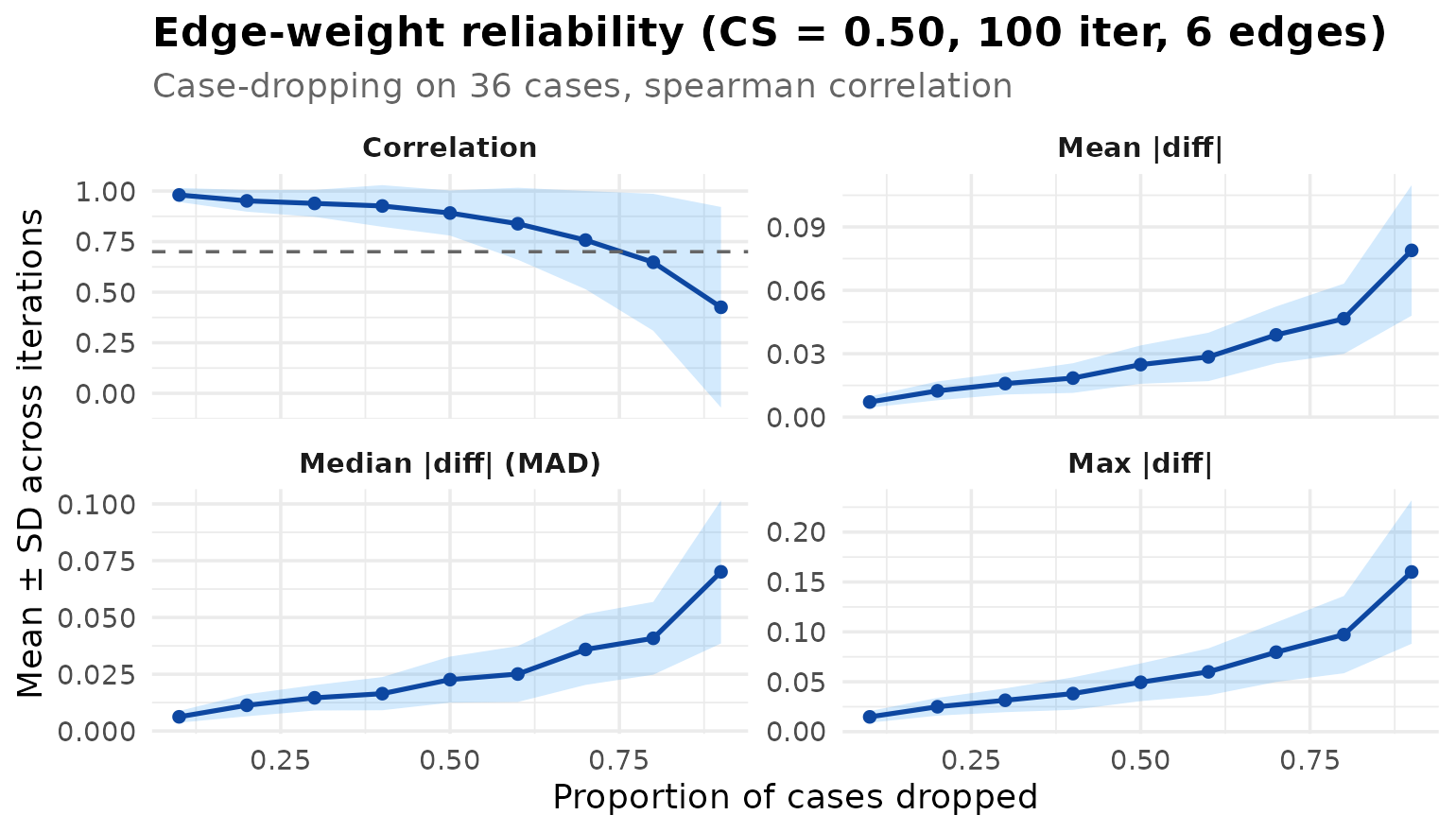

The verdicts are moderate across the board: the in-strength ordering holds to a 0.60 drop, the out-strength ordering only to 0.40, and the edge weights sit exactly at the 0.50 bar. This is what 36 sequences buy, and it is the sample-size counterweight to the posterior certainty above: report orderings and intervals, not bare point values.

Split-half reliability

set.seed(2026)
network_reliability(effort_model)
#> Split-Half Reliability (1000 iterations, split = 50%)
#>   Mean Abs. Diff.     mean = 0.0578  sd = 0.0220
#>   Median Abs. Diff.   mean = 0.0516  sd = 0.0240
#>   Pearson             mean = 0.8526  sd = 0.1147
#>   Max Abs. Diff.      mean = 0.1290  sd = 0.0509

Randomly halving the panel 1,000 times yields two models that correlate at 0.85 on average with a mean absolute edge difference of 0.06: real agreement, with real room for movement. All four verbs in this section tell the same story at different grain: the backbone of the model is solid, the weaker edges are not yet pinned down.

Comparing two models

Any two models on the same alphabet can be compared. The pair here splits the panel at occasion 78, the first and second halves of the course, with the same fixed breaks, so both models sit on one alphabet, and the same 36 students on both sides.

first_half <- ts_tna(
  subset(students, day <= 78),
  value = "effort", id = "name", time = "day",
  discretization = "threshold", breaks = c(40, 70),
  labels = c("low", "moderate", "high")
)

second_half <- ts_tna(
  subset(students, day > 78),
  value = "effort", id = "name", time = "day",
  discretization = "threshold", breaks = c(40, 70),
  labels = c("low", "moderate", "high")
)

The difference itself

subtract_networks() returns the edge-by-edge difference as an object cograph can draw:

half_difference <- subtract_networks(first_half, second_half)

half_difference
#> Network difference (x - y): 3 nodes, 9 differing edges
#> Plot: cograph::splot(d) or cograph::plot_difference(d)
#> 
#>      from       to         x         y    difference
#>       low moderate 0.3293592 0.2967836  0.0325755397
#>       low     high 0.2563338 0.2880117 -0.0316778658
#>      high moderate 0.2476273 0.2700348 -0.0224075783
#>      high     high 0.5858499 0.5662021  0.0196477800
#>  moderate      low 0.2134472 0.2230523 -0.0096051227
#>  moderate     high 0.3308431 0.3255069  0.0053361793
#>  moderate moderate 0.4557097 0.4514408  0.0042689434
#>      high      low 0.1665229 0.1637631  0.0027597983
#>       low      low 0.4143070 0.4152047 -0.0008976739

cograph::plot_difference(half_difference)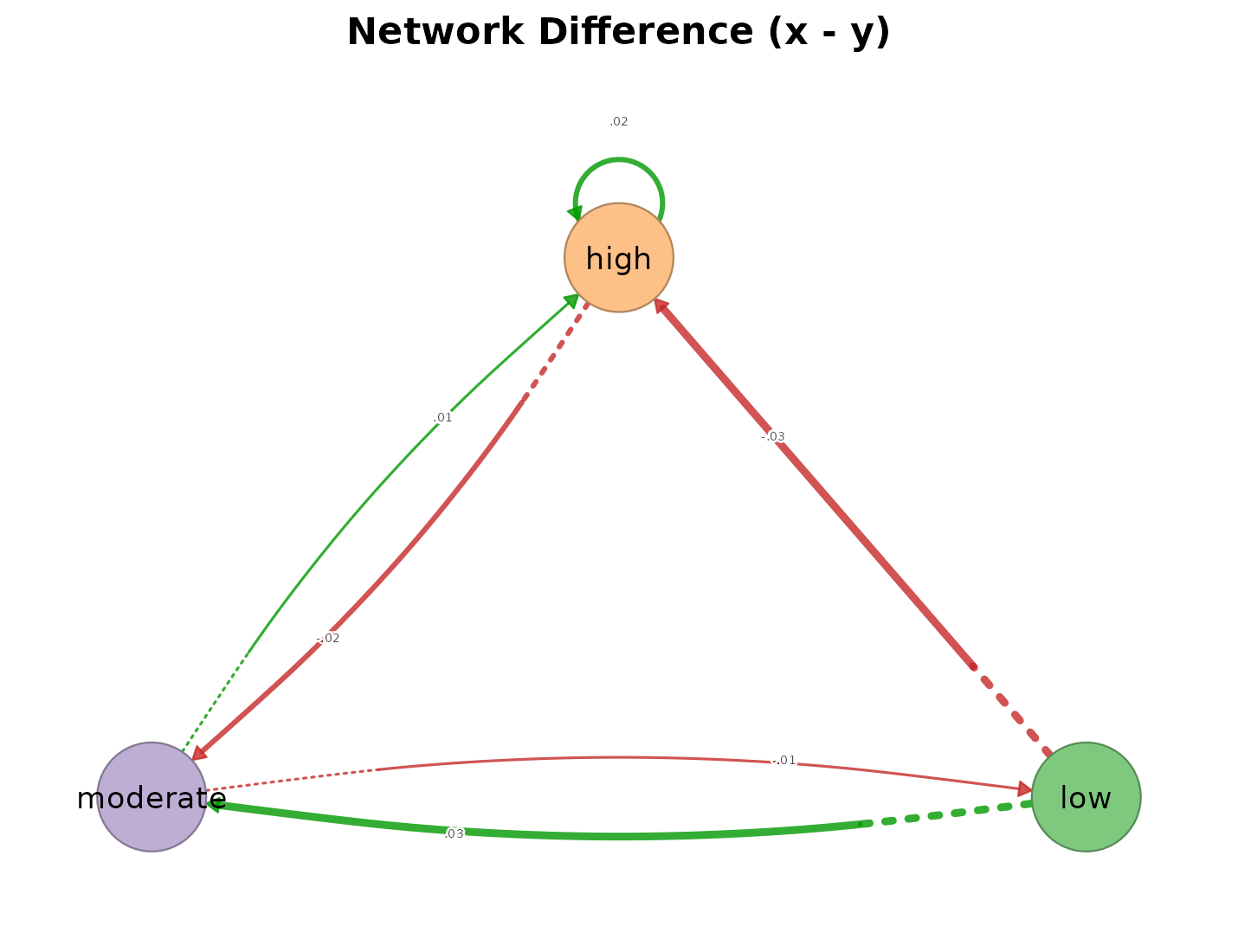

The largest gap on any edge is 0.033 (low → moderate).

Four more verdicts on the same pair

compare_model() condenses the pair into a metric panel; bayes_compare() asks whether each edge difference is credibly nonzero; vertex_compare() tests the network-level statistics; and the workflow vignette’s permutation() run supplies the sequence-level test.

half_panel <- compare_model(first_half, second_half)

half_panel
#> Network comparison
#> ==================
#> Summary metrics:
#>              category               metric    value
#>     Weight Deviations      Mean Abs. Diff.  0.01435
#>     Weight Deviations    Median Abs. Diff. 0.009605
#>     Weight Deviations            RMS Diff.  0.01856
#>     Weight Deviations       Max Abs. Diff.  0.03258
#>     Weight Deviations Rel. Mean Abs. Diff.  0.04306
#>     Weight Deviations             CV Ratio    1.069
#>          Correlations              Pearson   0.9904
#>          Correlations             Spearman        1
#>          Correlations              Kendall        1
#>          Correlations             Distance   0.9675
#>       Dissimilarities            Euclidean  0.05568
#>       Dissimilarities            Manhattan   0.1292
#>       Dissimilarities             Canberra   0.2148
#>       Dissimilarities          Bray-Curtis  0.02153
#>       Dissimilarities            Frobenius  0.04546
#>          Similarities               Cosine   0.9987
#>          Similarities              Jaccard   0.9578
#>          Similarities                 Dice   0.9785
#>          Similarities              Overlap   0.9785
#>          Similarities                   RV   0.9962
#>  Pattern Similarities       Rank Agreement        1
#>  Pattern Similarities       Sign Agreement        1
#> 
#> Network metrics (x vs y):
#>                       metric      x      y
#>                   Node Count      3      3
#>                   Edge Count      9      9
#>              Network Density      1      1
#>                Mean Distance 0.2574 0.2612
#>            Mean Out-Strength      1      1
#>              SD Out-Strength 0.1915 0.1895
#>             Mean In-Strength      1      1
#>               SD In-Strength      0      0
#>              Mean Out-Degree      3      3
#>                SD Out-Degree      0      0
#>  Centralization (Out-Degree)      0      0
#>   Centralization (In-Degree)      0      0
#>                  Reciprocity      1      1

plot(half_panel)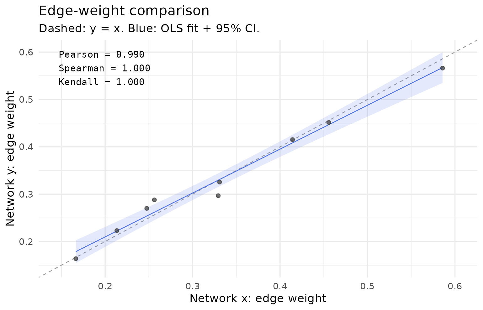

set.seed(2026)
bayes_compare(first_half, second_half)
#> Bayesian Dirichlet-Multinomial Comparison: Transition Network (relative probabilities) 
#>   Prior: Dirichlet(0.50)  |  Draws: 10000  |  CI: 95%
#>   Thresholds: |mean diff| > 0.010, nearest CI bound > 0.001
#>   Nodes: 3  |  Edges compared: 9  |  Credibly different: 0

vertex_compare(first_half, second_half, iter = 200, seed = 2026)
#> Two-Network Vertex Bootstrap Comparison (Snijders & Borgatti)
#>   x (3 nodes) vs y (3 nodes) | 200 replicates each
#> 
#>       statistic observed_x observed_y   diff se_diff      z p_value ci_lower
#>         density      1.000      1.000  0.000   0.000     NA      NA    0.000
#>     mean_weight      0.257      0.261 -0.004   0.028 -0.135   0.893   -0.060
#>  centralization      0.123      0.095  0.028   0.066  0.423   0.672   -0.101
#>     reciprocity      0.813      0.838 -0.025   0.070 -0.363   0.717   -0.163
#>  ci_upper sig
#>     0.000    
#>     0.052    
#>     0.157    
#>     0.112    
#> ---
#> Signif. codes: *** p<0.001, ** p<0.01, * p<0.05

Five verbs, one verdict. The matrices correlate at 0.990 with rank and sign agreement of 1; the posterior finds zero of nine edges credibly different; the vertex comparison finds no network-level statistic moved (all p ≥ 0.67); and the permutation test in the workflow vignette finds nothing at the sequence level either. The course’s second half reproduces its first, in level and in dynamics. When the verbs disagree, a posterior flagging tiny-but-credible differences that a sequence-level permutation absorbs, report the magnitude next to whichever test is used; the grouped weekday/weekend comparison in vignette("group-models", package = "tsn") shows what a real, localized difference looks like on these same students.

Link prediction

predict_links() scores unobserved dyads by six structural predictors:

predict_links(effort_model)
#> Link Prediction  [directed | weighted | 3 nodes | 6 existing edges]
#>   Methods: common_neighbors, resource_allocation, adamic_adar, jaccard, preferential_attachment, katz

It runs, but a three-state transition network is fully connected between states, which leaves link prediction nothing to rank; it earns its place on larger, pruned alphabets, where a missing edge is a real hypothesis.

Grouped models

When the comparison variable is a column of the data, ts_tna(group = ...) builds one network per level and returns a Nestimate netobject_group. The grouped verbs verified against it are net_centrality(), state_distribution(), transition_entropy(), passage_time(), certainty(), net_prune(), compare_model(), permutation(), bootstrap_network(), markov_order_test(), centrality_stability(), casedrop_reliability(), and mosaic_plot(); summary() and as.data.frame() return tidy per-group tables, and plot() draws one selected group. net_edge_betweenness() also runs, but its result drops back to a plain netobject_group. The dedicated vignette vignette("group-models", package = "tsn") works through all of it on the esm_srl weekday/weekend split.

What does not apply, and why

Three families of Nestimate verbs reject a transition model, each for a principled reason rather than a missing feature:

• Sequence-data verbs. frequencies(), mark_first_state(), mark_terminal_state(), entropy_trajectory(), mosaic_analysis(), plot_mosaic(), and as_htna() operate on a raw wide data frame of sequences, not on an estimated model. They belong before model construction in a workflow, applied to sequence data you hold yourself.
• Psychometric-network verbs. predictability() and the glasso/pcor/cor estimator family need a precision or correlation structure estimated from multivariate data. A transition matrix is a conditional-probability object, not a conditional-independence one; the quantities these verbs compute are undefined for it.
• Verbs that need extra structure. cluster_network() and build_clusters() require a chosen number of clusters and are aimed at multi-sequence typologies; wtna() needs one-hot action data; sequence_compare() wants sequence data plus a grouping vector. And as_tna() is unnecessary by design: a tsn model needs no conversion, which is the point of this vignette.

The compatibility map

Question	Verb	Tidy access	Plot	Notes
What are the estimates?	as.data.frame(), as.matrix(), extract_transition_matrix(), extract_initial_probs()	direct	via plot() on the model	tsn accessors include the diagonal
Between-state edges only	extract_edges()	direct	-	excludes self-transitions
Marginal composition	state_distribution(), state_frequencies()	data frame	mosaic_plot(), plot_state_frequencies()
Composition over time / carpet	distribution_plot(), sequence_plot()	-	draws directly	stacked area; sequence heatmap
State/edge importance	net_centrality(), net_edge_betweenness()	data frame / network	plot() on both	loops excluded from centrality by default
Travel times between states	passage_time()	print	plot()	Kemeny & Snell (1976)
Persistence, recurrence, sojourn	markov_stability()	$stability table	plot()
Chain diagnostics	chain_structure()	summary()	plot() heatmap	irreducibility, reversibility
Predictability	transition_entropy(), entropy_bayes(), entropy_network()	print / summary()	plot() on both entropy results	rate in bits; ceiling log2(n_states)
History beyond one step	markov_order_test(), path_dependence(), path_counts(), build_hon() + pathways()	print / data frame	plot() on test and dependence	test the size, not only the p
Simplification	net_prune(), net_pruning_details(), net_deprune()	same class back	via model plot()	prune after testing
Edge uncertainty	bootstrap_network(), certainty()	summary()	none	resampling vs Bayesian; they can disagree
Network-level uncertainty	vertex_bootstrap()	data frame	plot()	Snijders & Borgatti (1999)
Sample-size reliability	centrality_stability(), casedrop_reliability(), network_reliability()	print	plot() on all three	CS-coefficient bar: 0.5 / 0.7
Two-model comparison	permutation(), compare_model(), subtract_networks(), bayes_compare(), vertex_compare()	summary() / data frame	plot(); cograph::plot_difference()	report magnitudes with tests
Link prediction	predict_links()	print	none	needs a sparse alphabet to be informative
Many-group comparison	ts_tna(group=) + grouped verbs	as.data.frame()	plot(x, group=), mosaic_plot()	see vignette("group-models")
Rendering	plot(), cograph::splot()	none	none	requires cograph

References

Anderson, T. W., & Goodman, L. A. (1957). Statistical inference about Markov chains. The Annals of Mathematical Statistics, 28(1), 89–110.

Epskamp, S., Borsboom, D., & Fried, E. I. (2018). Estimating psychological networks and their accuracy: A tutorial paper. Behavior Research Methods, 50(1), 195–212.

Kemeny, J. G., & Snell, J. L. (1976). Finite Markov Chains. Springer.

Snijders, T. A. B., & Borgatti, S. P. (1999). Non-parametric standard errors and tests for network statistics. Connections, 22(2), 161–170.

Xu, J., Wickramarathne, T. L., & Chawla, N. V. (2016). Representing higher-order dependencies in networks. Science Advances, 2(5), e1600028.