Mean First Passage Times

Computes the full matrix of mean first passage times (MFPT) for a Markov chain. Element $M_{ij}$ is the expected number of steps to travel from state $i$ to state $j$ for the first time. The diagonal equals the mean recurrence time $1/\pi_i$.

Usage

passage_time(x, states = NULL, normalize = TRUE)

# S3 method for class 'net_mpt'
print(x, digits = 1, ...)

# S3 method for class 'net_mpt_group'
print(x, ...)

# S3 method for class 'net_mpt'
summary(object, ...)

# S3 method for class 'summary.net_mpt'
print(x, ...)

# S3 method for class 'net_mpt'
plot(
  x,
  log_scale = TRUE,
  digits = 1,
  title = "Mean First Passage Times",
  low = "#004d00",
  high = "#ccffcc",
  ...
)

Arguments

x: A netobject, cograph_network, tna object, row-stochastic numeric transition matrix, or a wide sequence data.frame (rows = actors, columns = time-steps; a relative transition network is built automatically). For the print() and plot() methods: an object of class net_mpt or net_mpt_group (or its summary()).
states: Character vector. Restrict output to these states. NULL (default) keeps all states.
normalize: Logical. If TRUE (default), rows that do not sum to 1 are normalized automatically (with a warning).
digits: Integer. Decimal places displayed in cells. Default 1.
...: Ignored. In plot.net_mpt(), print.net_mpt(), print.summary.net_mpt() and summary.net_mpt(): Ignored. In print.net_mpt_group(): Forwarded to print.net_mpt for each element.
object: A net_mpt object (for summary).
log_scale: Logical. Apply log transform to the fill scale for better contrast? Default TRUE.
title: Character. Plot title.
low: Character. Hex colour for the low end (short passage time). Default dark green "#004d00".
high: Character. Hex colour for the high end (long passage time). Default pale green "#ccffcc".

Value

An object of class "net_mpt" with:

matrix: Full $n \times n$ MFPT matrix. Row $i$, column $j$ = expected steps from state $i$ to state $j$. Diagonal = mean recurrence time $1/\pi_i$.
stationary: Named numeric vector: stationary distribution $\pi$.
return_times: Named numeric vector: $1/\pi_i$ per state.
states: Character vector of state names.

For a netobject_group the result is a "net_mpt_group": a named list holding one net_mpt per group.

In print.net_mpt(): x, invisibly.

In print.net_mpt_group(): x invisibly.

In summary.net_mpt(): summary.net_mpt returns an object of class "summary.net_mpt": a list whose table is a data frame with one row per state and columns state, return_time, stationary, mean_out (mean steps to other states) and mean_in (mean steps from other states), and whose object is the net_mpt it summarises. Its print method shows the table.

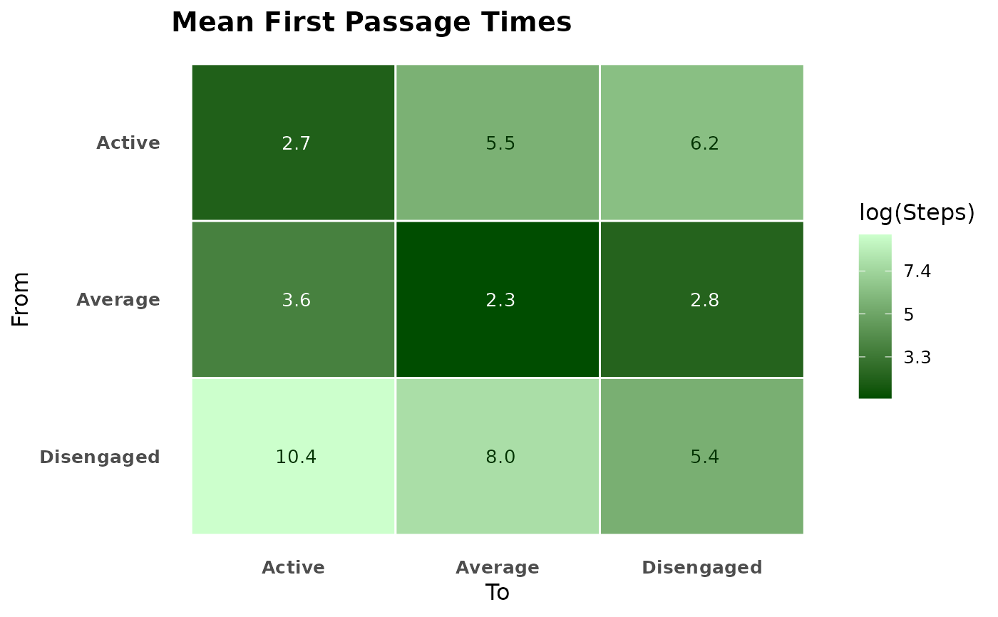
In plot.net_mpt(): plot.net_mpt returns a ggplot object: a from-by-to heatmap of the mean first passage time matrix.

In print.summary.net_mpt(): x, invisibly.

Details

Uses the Kemeny-Snell fundamental matrix formula: $$M_{ij} = \frac{Z_{jj} - Z_{ij}}{\pi_j}, \quad Z = (I - P + \Pi)^{-1}$$ where $\Pi_{ij} = \pi_j$. Requires an ergodic (irreducible, aperiodic) chain.

References

Kemeny, J.G. and Snell, J.L. (1976). Finite Markov Chains. Springer-Verlag.

Examples

net <- build_network(as.data.frame(trajectories), method = "relative")
pt  <- passage_time(net)
print(pt)
#> Mean First Passage Times (3 states)
#> 
#>            Active Average Disengaged
#> Active        2.7     3.6       10.4
#> Average       5.5     2.3        8.0
#> Disengaged    6.2     2.8        5.4
#> 
#> Stationary distribution:
#>     Active    Average Disengaged 
#>     0.3719     0.4431     0.1850 
# \donttest{
plot(pt)

# }