
Visualise state (node) frequency distributions across groups for any
Nestimate object that carries sequence data: a single netobject,
a netobject_group, an mcml model, or an htna network.
Usage
plot_state_frequencies(x, ...)

# S3 method for class 'nestimate_facet_plot'
print(x, ...)

# S3 method for class 'nestimate_facet_list'
print(x, ...)

# S3 method for class 'netobject'
plot_state_frequencies(
  x,
  style = "marimekko",
  metric = "prop",
  label = "prop",
  legend = "auto",
  legend_dir = "auto",
  legend_frame = "none",
  sort_states = "frequency",
  colors = NULL,
  label_size = 3.5,
  abbreviate = FALSE,
  include_macro = FALSE,
  combine = "auto",
  ncol = NULL,
  node_groups = NULL,
  ...
)

# S3 method for class 'htna'
plot_state_frequencies(
  x,
  style = "marimekko",
  metric = "prop",
  label = "prop",
  legend = "auto",
  legend_dir = "auto",
  legend_frame = "none",
  sort_states = "frequency",
  colors = NULL,
  label_size = 3.5,
  abbreviate = FALSE,
  include_macro = FALSE,
  combine = "auto",
  ncol = NULL,
  node_groups = NULL,
  ...
)

# S3 method for class 'mcml'
plot_state_frequencies(
  x,
  style = "marimekko",
  metric = "prop",
  label = "prop",
  legend = "auto",
  legend_dir = "auto",
  legend_frame = "none",
  sort_states = "frequency",
  colors = NULL,
  label_size = 3.5,
  abbreviate = FALSE,
  include_macro = FALSE,
  combine = "auto",
  ncol = NULL,
  node_groups = NULL,
  ...
)

# S3 method for class 'netobject_group'
plot_state_frequencies(
  x,
  style = "marimekko",
  metric = "prop",
  label = "prop",
  legend = "auto",
  legend_dir = "auto",
  legend_frame = "none",
  sort_states = "frequency",
  colors = NULL,
  label_size = 3.5,
  abbreviate = FALSE,
  include_macro = FALSE,
  combine = "auto",
  ncol = NULL,
  node_groups = NULL,
  ...
)

# Default S3 method
plot_state_frequencies(x, ...)

# S3 method for class 'state_freq'
print(x, digits = 1, max_states = 20L, ...)

# S3 method for class 'state_freq'
plot(x, ...)

# S3 method for class 'state_freq'
as.data.frame(x, ...)
Arguments
- x
A
netobject,netobject_group,mcml, orhtnaobject. For theprint(),plot()andas.data.frame()methods: thestate_freqobject returned byplot_state_frequencies(); for theprint()methods of the per-facet figure, an object of classnestimate_facet_plotornestimate_facet_list.- ...
Reserved for future use. In
as.data.frame.state_freq(),plot.state_freq(),print.state_freq(),print.nestimate_facet_list()andprint.nestimate_facet_plot(): ignored.- style
One of:
"marimekko"(default) – per-group treemap panels with cumulative-width geometry; tile area = within-group state share."bars"– horizontal bars sorted by frequency, faceted per group.
For chi-square mosaics of a (group x state) contingency table, use
mosaic_plotdirectly – it is kept as a separate function with its own dispatch surface.- metric
For
style = "bars": which value the bar length encodes –"prop"(default) or"freq". Treemap and hierarchical-marimekko areas always encode proportion within group.- label
Inline tile / bar annotation. All formats render on a single line.
"prop"(default) – proportion only, e.g."66%""freq"– count only, e.g."1,234""both"– count + proportion, e.g."1,234 (66%)""state"– state name only, e.g."Average""all"– state + proportion, e.g."Average (66%)""none"– no inline labels
- legend
Legend position.
"auto"(default) resolves per style:"none"forstyle = "bars"(the y-axis already names every state, so a colour legend is redundant);"per_facet"forhtna/mcmltreemaps (state vocabularies differ per panel, so each gets its own legend);"bottom"for single-network andnetobject_grouptreemaps (shared state vocabulary, one shared legend). Override with any of"bottom","top","right","left","none", or"per_facet"."per_facet"is silently demoted to"bottom"when every group shares the same state vocabulary (repeating one legend per panel would be redundant); when it does take effect it returns agtable(requiring the gridExtra package) or a list of ggplots, percombine.- legend_dir
Legend internal layout:
"auto"(default – horizontal for top/bottom, vertical for left/right), or force"horizontal"or"vertical"regardless of position.- legend_frame
"none"(default) for an unframed legend, or"border"to draw a thin grey rectangle around the legend ("legend enclosed in a square").- sort_states
One of
"frequency"(default – most frequent first),"alpha", or"none".- colors
Optional colors overriding the default Okabe-Ito state palette. Either an unnamed vector applied in state order (length at least the number of unique states), or a named lookup (
c(plan = "#0072B2")) overriding only the states you name.- label_size
Numeric size of inline labels (max size when ggfittext is installed – text auto-shrinks per tile).
- abbreviate
Abbreviate state names.
FALSE(default) shows full names;TRUEtruncates to the first 3 characters viabase::abbreviate()(which extends the truncation as needed to keep names unique after collision); a positive integer sets the target minimum length explicitly (e.g.abbreviate = 4). Affects tile labels, the legend, and the tidy table returned byas.data.frame().- include_macro
For
mcmlonly: prepend a"macro"reference column showing aggregate state frequencies across all clusters. DefaultFALSE.- combine
For
legend = "per_facet"only."auto"(default) returns a single combined gtable for 1-3 panels and a list of ggplots (one per panel) for 4+ panels – many-clustermcmllayouts read better as separate figures than as a tile grid.TRUEforces a combined gtable via gridExtra;FALSEforces a list (knitr renders each at the chunk's fullfig.width/fig.height).- ncol
For
legend = "per_facet"withcombine = TRUE: number of columns in the grid arrangement.NULL(default) picks 1, 2, or 3 columns based on the number of panels.- node_groups
Optional named character vector mapping node labels to semantic groups. When supplied, panels (or bars) are coloured / annotated by group rather than by individual state, so state-level palettes can collapse onto a smaller categorical legend.
- digits
Number of decimal places for proportion / share columns. Default 1.
- max_states
Cap on rows shown per group in the per-state table (default 20); the surplus is folded into a single
"(+k more)"row. The full, uncapped table is returned byas.data.frame(x).
Value
A state_freq object: a list with the rendered $plot
(a ggplot; a gtable or a list of ggplots under
legend = "per_facet", per combine), the tidy $table (a
data.frame with columns group, state, count,
proportion, one row per (group, state) cell), and the call's
$style, $metric, $source_class. The class supports
print() (prints the tidy table and draws the chart),
plot() (draws the chart alone), and as.data.frame()
(returns the tidy table) – see the section below.
print() returns x invisibly (after printing the
table and drawing the chart); plot() returns invisible(NULL)
after drawing; as.data.frame() returns the tidy
data.frame, one row per (group, state) cell with columns
group, state, count, proportion.
Details
The marimekko layout is dispatched per class:
For
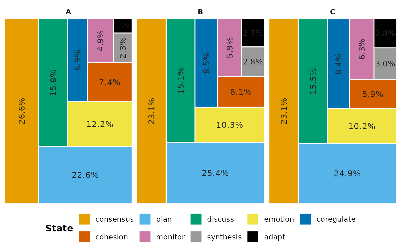
mcml, where states partition cleanly into clusters, the chart is a hierarchical 2D marimekko: cluster columns of width proportional to cluster total, segments stacked vertically with heights proportional to within-cluster state proportions.For all other classes (
netobject,netobject_group,htna), each group is rendered as its own panel containing a squarified treemap: each state becomes a rectangular tile whose AREA is exactly proportional to the state's share within that group. Single-panel when no groups exist; faceted when groups are present.
The bar style produces horizontal bars (state on the y-axis), faceted by group when groups exist. All variants use the Okabe-Ito palette.
The state_freq object
plot_state_frequencies() returns a state_freq object holding
both the rendered chart and the tidy frequency table. print() shows
the table in the console and draws the chart on the active graphics
device, plot() draws the chart alone, and as.data.frame()
returns the tidy table for downstream piping.
Examples
if (requireNamespace("ggplot2", quietly = TRUE)) {
data(group_regulation_long, package = "Nestimate")
nw <- build_network(group_regulation_long,
method = "relative", format = "long",
actor = "Actor", action = "Action",
order = "Time", group = "Course")
res <- plot_state_frequencies(nw)
print(res) # tidy frequency table in the console
plot(res) # ggplot chart
head(as.data.frame(res))
}
#> State frequencies (style = marimekko, source = netobject_group)
#> Total events: 27,533 | Groups: 3 | States: 9
#>
#> Per-group totals
#> group events share
#> A 12,390 45.0%
#> B 9,626 35.0%
#> C 5,517 20.0%
#>
#> Per-state proportions (within group)
#> group state count share
#> A consensus 3,298 26.6%
#> A plan 2,805 22.6%
#> A discuss 1,960 15.8%
#> A emotion 1,517 12.2%
#> A cohesion 923 7.4%
#> A coregulate 855 6.9%
#> A monitor 602 4.9%
#> A synthesis 290 2.3%
#> A adapt 140 1.1%
#> B plan 2,445 25.4%
#> B consensus 2,226 23.1%
#> B discuss 1,453 15.1%
#> B emotion 995 10.3%
#> B coregulate 817 8.5%
#> B cohesion 590 6.1%
#> B monitor 565 5.9%
#> B synthesis 274 2.8%
#> B adapt 261 2.7%
#> C plan 1,373 24.9%
#> C consensus 1,273 23.1%
#> C discuss 854 15.5%
#> C emotion 563 10.2%
#> C coregulate 461 8.4%
#> C monitor 349 6.3%
#> C cohesion 326 5.9%
#> C synthesis 165 3.0%
#> C adapt 153 2.8%
 #> group state count proportion
#> 1 A consensus 3298 0.26618241
#> 2 A plan 2805 0.22639225
#> 3 A discuss 1960 0.15819209
#> 4 A emotion 1517 0.12243745
#> 5 A cohesion 923 0.07449556
#> 6 A coregulate 855 0.06900726
#> group state count proportion
#> 1 A consensus 3298 0.26618241
#> 2 A plan 2805 0.22639225
#> 3 A discuss 1960 0.15819209
#> 4 A emotion 1517 0.12243745
#> 5 A cohesion 923 0.07449556
#> 6 A coregulate 855 0.06900726