State Distribution Plot Over Time

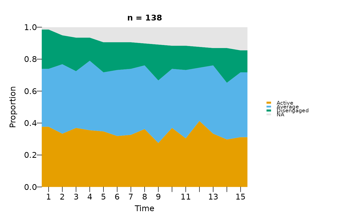
Draws how state proportions (or counts) evolve across time points. For each time column, tabulates how many sequences are in each state and renders the result as a stacked area (default) or stacked bar chart. Accepts the same inputs as sequence_plot.

Usage

distribution_plot(
  x,
  group = NULL,
  scale = c("proportion", "count"),
  geom = c("area", "bar"),
  na = TRUE,
  trim = NULL,
  trim_clusterwise = FALSE,
  state_colors = NULL,
  na_color = "grey90",
  frame = FALSE,
  width = NULL,
  height = NULL,
  main = NULL,
  show_n = TRUE,
  time_label = "Time",
  xlab = NULL,
  y_label = NULL,
  ylab = NULL,
  tick = NULL,
  ncol = NULL,
  nrow = NULL,
  combined = TRUE,
  legend = c("right", "bottom", "none"),
  legend_size = NULL,
  legend_title = NULL,
  legend_ncol = NULL,
  legend_border = NA,
  legend_bty = "n"
)

Arguments

x: Wide-format sequence data. Accepts the same inputs as sequence_plot: data.frame, matrix, netobject, net_clustering, netobject_group, net_mmm, or tna. When clustering info is available, one panel is drawn per cluster.
group: Optional grouping vector (length nrow(x)) producing one panel per group. Ignored if x is a net_clustering.
scale: "proportion" (default) divides each column by its total so bands fill 0..1. "count" keeps raw counts.
geom: "area" (default) draws stacked polygons; "bar" draws stacked bars.
na: If TRUE (default), NA cells are shown as an extra band coloured na_color.
trim: Optional time-axis truncation, to stop a few long sequences from stretching the plot. NULL (default) keeps the full width. A fraction in (0, 1) drops everything past that quantile of sequence lengths (e.g. trim = 0.95); a value >= 1 is an absolute cut (trim = 50 keeps the first 50 time points). See sequence_plot.
trim_clusterwise: Grouped plots only, fractional trim only. FALSE (default) uses one pooled cutoff for every panel so the time axes stay aligned; TRUE crops each group to its own length quantile (panels can differ in width). See sequence_plot.
state_colors: Vector of colours, one per state. Defaults to Okabe-Ito.
na_color: Colour for the NA band.
frame: If TRUE (default), draw a box around each panel.
width, height: Optional device dimensions. See sequence_plot.
main: Plot title.
show_n: Append "(n = N)" (per-group when grouped) to the title.
time_label: X-axis label.
xlab: Alias for time_label.
y_label: Y-axis label. Defaults to "Proportion" or "Count" based on scale.
ylab: Alias for y_label.
tick: Show every Nth x-axis label. NULL = auto.
ncol, nrow: Facet grid dimensions. NULL = auto: ncol = ceiling(sqrt(G)), nrow = ceiling(G / ncol). Ignored when combined = FALSE.
combined: When TRUE (default), groups are arranged on one figure via graphics::layout(). When FALSE, each group is drawn on its own page (one full-size figure per group, with its own legend). Useful when you want each group at full size in knitr (fig.show = "asis") or to save each as a separate file. Single-group calls (G == 1) ignore this argument.
legend: Legend position: "right" (default), "bottom", or "none".
legend_size: Legend text size. NULL (default) auto-scales from device width (clamped to [0.65, 1.2]).
legend_title: Optional legend title.
legend_ncol: Number of legend columns.
legend_border: Swatch border colour.
legend_bty: "n" (borderless) or "o" (boxed).

Value

Invisibly, a list with counts, proportions, levels, palette, and groups.

Examples

# \donttest{
distribution_plot(as.data.frame(trajectories))

# }

Usage

Arguments

Value

See also

Examples