entropy_bayes() puts credible intervals on the entropy quantities of
transition_entropy() and on the edge-level decomposition of
entropy_network(). Each row of the transition count matrix gets an
independent Dirichlet posterior (counts + prior), and Monte Carlo draws
from it carry the uncertainty of the counts into the entropy rate, the
stationary entropy, the redundancy, each state's branching entropy and
stationary probability, and every edge's entropy contribution. Each is
reported as a posterior mean with an equal-tailed credible interval. The
counts are recovered from a network, a tna model, a count matrix or
sequence data (see x); a netobject_group gives one result per group.
The practical purpose is to exclude unstable estimates: an edge
whose contribution rests on a handful of observations has a wide
posterior, and it is flagged as not credible unless it credibly accounts
for at least min_share of the entropy rate. The pruned network keeps the
credible edges only, the stable entropy skeleton. The posterior treats
every transition as an independent draw from its row of a first-order
chain; whether a first-order chain describes the sequences is a separate
question, which markov_order_test() tests.
Usage
entropy_bayes(
  x,
  prior = 0.5,
  draws = 4000,
  ci = 0.95,
  min_share = 0.01,
  base = 2,
  seed = NULL
)

# S3 method for class 'net_entropy_bayes'
print(x, digits = 3, ...)

# S3 method for class 'net_entropy_bayes_group'
print(x, ...)

# S3 method for class 'net_entropy_bayes_group'
summary(object, ...)

# S3 method for class 'net_entropy_bayes_group'
plot(x, top = 25, title = paste("Bayesian edge entropy", "contributions"), ...)

# S3 method for class 'net_entropy_bayes'
summary(object, ...)

# S3 method for class 'net_entropy_bayes'
plot(x, top = 25, title = "Bayesian edge entropy contributions", ...)
Arguments
- x
The transition counts: a frequency
netobject(build_network(method = "frequency")); a relative, frequency or co-occurrencenetobjectthat carries its data, recounted with the network's own start and end states, concatenation, windows and one-hot units; a one-hot network built withbuild_network(method = "wtna")or"wtna_cooccurrence", with its data, recounted the same way (awtna()result, whose method is"wtna_transition", currently raisesnestimate_bad_input); an unscaled frequency, co-occurrence or reverse network without data, whose weights are the counts; a network without a declared method whose weights are non-negative whole numbers, read as counts; atnamodel; a count matrix (non-negative whole numbers); or wide sequence data (a data frame or a character matrix) that holds a numbered run of positions (T1, T2, ...), from which a frequency network is built, other columns set aside with a message. For a frame without such a run, pass a network built withbuild_network(). When a network declares its method, counts are read from that method, never from the values: a scaled or relative network is recounted from its data. An association network, or any other network whose counts cannot be recovered, raises an error of classnestimate_bad_input; a matrix of probabilities raises an error. Anetobject_groupgives one result per group. For theprint()andplot()methods: anentropy_bayes()result;print()also takes a group result.- prior
The Dirichlet concentration added to every cell of the count matrix, a positive number. Default
0.5(Jeffreys).- draws
The number of Monte Carlo posterior draws, at least 100. Default
4000.- ci
The mass of the credible intervals, between 0 and 1. Default
0.95.The credibility threshold, a proportion in \([0, 1)\): an edge is credible when the lower limit of the credible interval of its share of the entropy rate exceeds it. Default
0.01: the edge credibly accounts for at least 1% of the entropy rate.- base
The logarithm base, which sets the unit:
2(default) for bits. Any positive number other than 1.- seed
An integer that makes the draws reproducible. Default
NULL. The session's own random stream is left as it was; a group uses the same seed for every group.- digits
For
print()of a result: decimal places of the chain-level estimates. Default3. A group result prints with three.- ...
- object
For
summary(): anentropy_bayes()result.- top
For
plot(): the most edges to show, those with the largest posterior mean contribution. Default25.- title
For
plot(): the plot title. Default"Bayesian edge entropy contributions".
Value
A net_entropy_bayes object, or for a netobject_group a
net_entropy_bayes_group: a named list of them, one per group.
print() shows the posterior mean and credible interval of the entropy
rate, stationary entropy and redundancy, and how many edges are
credible; for a group, each group's entropy rate. For a group,
summary() returns the chain-level table of every group stacked, with a
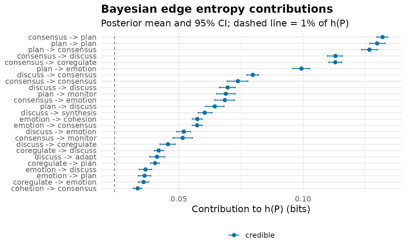
group column, and plot() draws the forest plot below in one panel
per group. For one network, summary() prints the
chain-level table and the per-edge table and returns the per-edge data
frame invisibly. plot() returns a ggplot forest plot of the edges
with the largest posterior mean contributions: the mean and credible
interval of each, credible edges in Okabe-Ito blue and unstable ones in
grey, with a dashed line at min_share of the posterior mean entropy
rate, the stability criterion. The print() methods return their input
invisibly. The object's fields:
- summary
Data frame, one row per chain-level quantity (
entropy_rate,stationary_entropy,redundancy), with the posteriormean,sd,ci_lowerandci_upper.- states
Data frame, one row per state: the posterior mean, sd and credible interval of its branching entropy, and the posterior mean and credible interval of its stationary probability.
- edges
Data frame, one row per observed transition (
from,to,count), sorted by contribution, largest first: the posterior mean, sd and credible interval of its contribution (inbaseunits), the posterior mean and credible interval of its share of the entropy rate (a proportion), and thecredibleflag.- network
A
netobject: the posterior-mean entropy network, every observed edge included, with the entropy edge style (vermilion edges, 2-digit labels, no minimum-weight pruning, node rings showing the posterior mean stationary distribution).- model
A
netobject: the pruned entropy network, posterior means wherecredibleand0elsewhere, styled the same way.- draws_entropy_rate
The posterior draws of the entropy rate, for further analysis or plotting.
- prior, draws, ci, min_share, base
The settings used.
- states_names
Character vector of state names.
Details
With prior > 0 the posterior puts mass on every transition, so the
contribution draws are strictly positive and a rule such as "the interval
excludes zero" would flag every edge as credible. The share criterion is
used instead: an edge is stable when it credibly carries at least
min_share of \(h(P)\). An unobserved transition (count 0) gets prior
mass only; it is left out of the edge table and of both networks.
The posterior mean entropy rate differs from the plug-in estimate of
transition_entropy() in two opposite ways: the prior pulls every row
toward uniform, which raises the entropy, and averaging over the posterior
lowers it. Which effect wins depends on the data (on the first 200 events of
group_regulation_long the posterior mean is above the plug-in value); the
difference is largest on sparse counts and vanishes as the counts grow.
Examples
net <- build_network(group_regulation_long, method = "relative",
                     actor = "Actor", action = "Action", time = "Time")
eb <- entropy_bayes(net, draws = 1000, seed = 1)
eb
#> Bayesian Transition Entropy (9 states, bits; Dirichlet prior 0.5, 1000 draws)
#>
#>   entropy_rate:       2.411 [2.396, 2.425]
#>   stationary_entropy: 2.783 [2.771, 2.796]
#>   redundancy:         0.373 [0.361, 0.384]
#>
#> Edges: 78 observed; 31 credible (share of h(P) credibly > 1%).
#> Use summary() for the edge table and plot() for the posterior.
summary(eb)
#> Chain-level posterior:
#>            quantity   mean     sd ci_lower ci_upper
#>        entropy_rate 2.4109 0.0074   2.3963   2.4250
#>  stationary_entropy 2.7834 0.0066   2.7710   2.7957
#>          redundancy 0.3726 0.0060   0.3612   0.3845
#>
#> Per-edge posterior (sorted by contribution):
#>        from         to count contribution     sd ci_lower ci_upper  share
#>   consensus       plan  2505       0.1320 0.0011   0.1297   0.1341 0.0547
#>        plan       plan  2304       0.1298 0.0017   0.1268   0.1330 0.0538
#>        plan  consensus  1788       0.1267 0.0017   0.1236   0.1300 0.0526
#>   consensus    discuss  1190       0.1130 0.0015   0.1099   0.1158 0.0469
#>   consensus coregulate  1188       0.1130 0.0014   0.1104   0.1156 0.0469
#>        plan    emotion   904       0.0993 0.0017   0.0959   0.1027 0.0412
#>     discuss  consensus  1269       0.0798 0.0012   0.0774   0.0821 0.0331
#>   consensus  consensus   519       0.0738 0.0021   0.0695   0.0778 0.0306
#>     discuss    discuss   770       0.0697 0.0016   0.0663   0.0727 0.0289
#>        plan    monitor   465       0.0689 0.0019   0.0652   0.0727 0.0286
#>   consensus    emotion   460       0.0685 0.0020   0.0645   0.0723 0.0284
#>        plan    discuss   418       0.0645 0.0019   0.0607   0.0682 0.0267
#>     discuss  synthesis   557       0.0604 0.0014   0.0578   0.0633 0.0251
#>     emotion   cohesion   923       0.0575 0.0010   0.0554   0.0594 0.0238
#>     emotion  consensus   909       0.0574 0.0010   0.0554   0.0594 0.0238
#>     discuss    emotion   418       0.0520 0.0015   0.0491   0.0547 0.0216
#>   consensus    monitor   295       0.0515 0.0020   0.0476   0.0554 0.0214
#>     discuss coregulate   333       0.0456 0.0015   0.0424   0.0485 0.0189
#>  coregulate    discuss   539       0.0419 0.0009   0.0401   0.0437 0.0174
#>     discuss      adapt   282       0.0412 0.0016   0.0383   0.0443 0.0171
#>  coregulate       plan   471       0.0404 0.0009   0.0386   0.0422 0.0168
#>     emotion    discuss   289       0.0366 0.0013   0.0341   0.0391 0.0152
#>     emotion       plan   283       0.0362 0.0013   0.0337   0.0387 0.0150
#>  coregulate    emotion   339       0.0358 0.0011   0.0337   0.0378 0.0149
#>    cohesion  consensus   844       0.0334 0.0008   0.0318   0.0351 0.0139
#>        plan   cohesion   155       0.0328 0.0019   0.0292   0.0367 0.0136
#>  coregulate  consensus   265       0.0319 0.0011   0.0298   0.0342 0.0132
#>     discuss   cohesion   188       0.0317 0.0016   0.0284   0.0349 0.0132
#>     emotion    emotion   218       0.0310 0.0015   0.0282   0.0338 0.0129
#>    cohesion       plan   239       0.0265 0.0009   0.0247   0.0283 0.0110
#>     monitor    discuss   538       0.0259 0.0007   0.0245   0.0272 0.0107
#>  coregulate    monitor   170       0.0250 0.0012   0.0227   0.0274 0.0104
#>        plan coregulate   106       0.0248 0.0018   0.0212   0.0285 0.0103
#>    cohesion coregulate   202       0.0244 0.0010   0.0224   0.0263 0.0101
#>    cohesion    emotion   196       0.0240 0.0010   0.0218   0.0258 0.0099
#>     monitor       plan   309       0.0233 0.0007   0.0219   0.0247 0.0097
#>   consensus   cohesion    94       0.0225 0.0018   0.0191   0.0260 0.0093
#>     monitor  consensus   228       0.0206 0.0008   0.0190   0.0221 0.0085
#>     emotion    monitor   103       0.0190 0.0013   0.0163   0.0216 0.0079
#>     discuss    monitor    88       0.0186 0.0015   0.0159   0.0215 0.0077
#>     emotion coregulate    97       0.0182 0.0013   0.0157   0.0205 0.0075
#>    cohesion    discuss   101       0.0162 0.0011   0.0142   0.0184 0.0067
#>     monitor    emotion   130       0.0153 0.0008   0.0136   0.0169 0.0063
#>  coregulate   cohesion    71       0.0143 0.0012   0.0120   0.0167 0.0059
#>   synthesis  consensus   304       0.0137 0.0005   0.0127   0.0148 0.0057
#>   consensus  synthesis    48       0.0134 0.0015   0.0105   0.0164 0.0055
#>   synthesis      adapt   153       0.0131 0.0006   0.0120   0.0142 0.0054
#>     monitor coregulate    83       0.0117 0.0009   0.0101   0.0133 0.0048
#>     monitor   cohesion    80       0.0113 0.0009   0.0097   0.0131 0.0047
#>     discuss       plan    46       0.0113 0.0013   0.0090   0.0139 0.0047
#>    cohesion    monitor    56       0.0109 0.0010   0.0089   0.0130 0.0045
#>       adapt   cohesion   139       0.0107 0.0005   0.0098   0.0116 0.0044
#>       adapt  consensus   243       0.0107 0.0005   0.0098   0.0116 0.0044
#>  coregulate coregulate    46       0.0104 0.0012   0.0082   0.0129 0.0043
#>    cohesion   cohesion    46       0.0094 0.0010   0.0075   0.0113 0.0039
#>   consensus      adapt    30       0.0092 0.0014   0.0068   0.0120 0.0038
#>  coregulate  synthesis    37       0.0089 0.0011   0.0070   0.0111 0.0037
#>  coregulate      adapt    32       0.0080 0.0011   0.0060   0.0101 0.0033
#>       adapt    emotion    61       0.0077 0.0006   0.0065   0.0088 0.0032
#>   synthesis       plan    49       0.0075 0.0007   0.0063   0.0088 0.0031
#>   synthesis    emotion    46       0.0072 0.0007   0.0058   0.0085 0.0030
#>   synthesis    discuss    41       0.0067 0.0007   0.0055   0.0083 0.0028
#>   synthesis coregulate    29       0.0053 0.0007   0.0041   0.0067 0.0022
#>     monitor    monitor    26       0.0052 0.0007   0.0038   0.0067 0.0021
#>       adapt    discuss    30       0.0050 0.0006   0.0039   0.0062 0.0021
#>     monitor  synthesis    23       0.0047 0.0007   0.0033   0.0062 0.0020
#>   synthesis   cohesion    22       0.0045 0.0007   0.0033   0.0058 0.0018
#>        plan  synthesis    11       0.0041 0.0010   0.0023   0.0063 0.0017
#>     monitor      adapt    16       0.0036 0.0007   0.0024   0.0050 0.0015
#>       adapt    monitor    17       0.0035 0.0006   0.0024   0.0046 0.0014
#>     emotion  synthesis     8       0.0027 0.0007   0.0014   0.0042 0.0011
#>       adapt coregulate    11       0.0025 0.0006   0.0015   0.0037 0.0011
#>        plan      adapt     6       0.0025 0.0008   0.0011   0.0043 0.0010
#>     emotion      adapt     7       0.0024 0.0007   0.0012   0.0040 0.0010
#>   synthesis    monitor     8       0.0022 0.0006   0.0011   0.0035 0.0009
#>    cohesion  synthesis     6       0.0020 0.0007   0.0009   0.0034 0.0008
#>       adapt       plan     8       0.0020 0.0005   0.0010   0.0032 0.0008
#>    cohesion      adapt     5       0.0018 0.0006   0.0007   0.0031 0.0007
#>  share_lower share_upper credible
#>       0.0537      0.0557     TRUE
#>       0.0523      0.0554     TRUE
#>       0.0511      0.0541     TRUE
#>       0.0456      0.0481     TRUE
#>       0.0457      0.0481     TRUE
#>       0.0397      0.0427     TRUE
#>       0.0321      0.0340     TRUE
#>       0.0288      0.0323     TRUE
#>       0.0275      0.0301     TRUE
#>       0.0270      0.0302     TRUE
#>       0.0268      0.0300     TRUE
#>       0.0252      0.0283     TRUE
#>       0.0240      0.0262     TRUE
#>       0.0230      0.0246     TRUE
#>       0.0230      0.0246     TRUE
#>       0.0204      0.0227     TRUE
#>       0.0197      0.0230     TRUE
#>       0.0176      0.0201     TRUE
#>       0.0166      0.0181     TRUE
#>       0.0159      0.0184     TRUE
#>       0.0160      0.0175     TRUE
#>       0.0141      0.0162     TRUE
#>       0.0140      0.0161     TRUE
#>       0.0140      0.0157     TRUE
#>       0.0132      0.0145     TRUE
#>       0.0121      0.0152     TRUE
#>       0.0124      0.0142     TRUE
#>       0.0118      0.0145     TRUE
#>       0.0117      0.0140     TRUE
#>       0.0102      0.0117     TRUE
#>       0.0102      0.0112     TRUE
#>       0.0094      0.0114    FALSE
#>       0.0088      0.0118    FALSE
#>       0.0093      0.0109    FALSE
#>       0.0091      0.0107    FALSE
#>       0.0091      0.0102    FALSE
#>       0.0079      0.0108    FALSE
#>       0.0079      0.0092    FALSE
#>       0.0068      0.0090    FALSE
#>       0.0066      0.0089    FALSE
#>       0.0065      0.0085    FALSE
#>       0.0059      0.0076    FALSE
#>       0.0057      0.0070    FALSE
#>       0.0050      0.0069    FALSE
#>       0.0053      0.0061    FALSE
#>       0.0044      0.0068    FALSE
#>       0.0050      0.0059    FALSE
#>       0.0042      0.0055    FALSE
#>       0.0040      0.0054    FALSE
#>       0.0037      0.0058    FALSE
#>       0.0037      0.0054    FALSE
#>       0.0040      0.0048    FALSE
#>       0.0041      0.0048    FALSE
#>       0.0034      0.0053    FALSE
#>       0.0031      0.0047    FALSE
#>       0.0028      0.0050    FALSE
#>       0.0029      0.0046    FALSE
#>       0.0025      0.0042    FALSE
#>       0.0027      0.0036    FALSE
#>       0.0026      0.0036    FALSE
#>       0.0024      0.0035    FALSE
#>       0.0023      0.0034    FALSE
#>       0.0017      0.0028    FALSE
#>       0.0016      0.0028    FALSE
#>       0.0016      0.0026    FALSE
#>       0.0014      0.0026    FALSE
#>       0.0014      0.0024    FALSE
#>       0.0009      0.0026    FALSE
#>       0.0010      0.0021    FALSE
#>       0.0010      0.0019    FALSE
#>       0.0006      0.0018    FALSE
#>       0.0006      0.0015    FALSE
#>       0.0004      0.0018    FALSE
#>       0.0005      0.0016    FALSE
#>       0.0005      0.0015    FALSE
#>       0.0004      0.0014    FALSE
#>       0.0004      0.0013    FALSE
#>       0.0003      0.0013    FALSE
plot(eb)