Principled test of whether a categorical sequence is best described
as a \(k\)-th order Markov chain. At each order
\(k = 1, \ldots,\) max_order, the function computes the
classical likelihood-ratio statistic (\(G^2\)) for the conditional
independence \(s \perp x \mid w\), where \(w\) is the
\((k-1)\)-gram context, \(x\) is the extra (k-th-back) state
added at order \(k\), and \(s\) is the next state. Under
\(H_0\) (order-\((k-1)\) is correct), \(s\) is independent of
\(x\) given \(w\).
The null distribution is obtained by an exact within-\(w\) permutation test: for each context \(w\) the successor labels are exchangeable under \(H_0\), so shuffling \(s\) within each \(w\)-group yields an exact reference distribution for \(G^2\). No plug-in MLE bias and no refitting per replicate. An asymptotic \(\chi^2\) p-value is reported alongside for reference.
Order selection is sequential: the order is raised while the test
rejects, and stops at the first non-rejection. The reported
optimal_order is therefore the highest \(k\) whose test - and
every test below it - rejected at level alpha, i.e. one below the
first non-rejection; it is 0 when order 1 is already not
rejected, and max_order when no test accepts.
Usage
markov_order_test(
  data,
  max_order = 3L,
  n_perm = 500L,
  alpha = 0.05,
  parallel = FALSE,
  n_cores = 2L,
  seed = NULL
)

# S3 method for class 'net_markov_order'
print(x, ...)

# S3 method for class 'net_markov_order_group'
print(x, ...)

# S3 method for class 'net_markov_order'
summary(object, ...)

# S3 method for class 'net_markov_order'
plot(x, panel = c("both", "ic", "permutation"), combined = TRUE, ...)
Arguments
- data
A data.frame (wide format, one sequence per row), a list of character vectors (one per trajectory), a
netobjectornetobject_groupcarrying its$data, or aprepareresult (itssequence_datais used). NAs are treated as end of sequence.- max_order
Integer. Highest Markov order to test. Default 3.
- n_perm
Integer. Number of within-\(w\) permutations per order. Default 500.
- alpha
Numeric. Significance level for order selection. Default 0.05.
- parallel
Logical. Use
parallel::mclapplyfor permutations. DefaultFALSE(setTRUEonly on Unix-like systems).- n_cores
Integer. Cores for parallel execution. Default 2.
- seed
Optional integer seed for reproducibility.
- x
For the
print()andplot()methods: an object of classnet_markov_orderornet_markov_order_group.- ...
In
plot.net_markov_order(),print.net_markov_order()andsummary.net_markov_order(): Ignored. Inprint.net_markov_order_group(): Forwarded toprint.net_markov_orderfor each element.- object
For the
summary()method: an object of classnet_markov_order.- panel
Which panel(s) to render:
"both","ic", or"permutation". Default"both".- combined
When
panel = "both"andcombined = TRUE(default), the two panels are drawn side-by-side. If gridExtra is installed they are arranged into a single drawable/saveable gtable (returned); otherwise basegridviewports draw both panels and a named list of the two ggplots is returned invisibly. WhenFALSE, returns that named list (ic,permutation) without drawing. Ignored whenpanel != "both".
Value
An object of class net_markov_order with elements:
- optimal_order
Integer. Selected order via sequential permutation test.
- bic_order
Integer. Order minimising BIC (reported by
print/plot; not used in the permutation selection).- aic_order
Integer. Order minimising AIC (reported by
print/plot; not used in the permutation selection).- test_table
Tidy data.frame, one row per order tested with columns
order,loglik,AIC,BIC,df,g2,p_permutation,p_asymptotic,significant.AIC/BICare the information-criterion values used for theicplot panel and to deriveaic_order/bic_order; the order-0 row hasNAfor the test columns (df,g2,p_permutation,p_asymptotic,significant).- permutation_null
List of numeric vectors (length
max_order), one empirical null \(G^2\) distribution per order.- logliks
Named numeric vector of log-likelihoods per order (for AIC / BIC panel only, not used in the test).
- layer_dofs
Named integer vector of model degrees of freedom per order (free parameters added at each layer), used to compute the AIC / BIC columns.
- transition_matrices
List of fitted transition matrices.
- states
Character vector of observed state labels.
- n_sequences, n_observations
Data summary.
- n_perm, alpha, max_order
Call settings.
max_orderis the order actually tested, which is capped atlength(longest sequence) - 1with a message.
For a netobject_group the result is a
"net_markov_order_group": a named list holding one
net_markov_order per group.
In print.net_markov_order(): The input object, invisibly.
In print.net_markov_order_group(): x invisibly.
In summary.net_markov_order(): The tidy test_table data.frame - one row per order tested - carrying the selection context as attributes: optimal_order, bic_order, aic_order, alpha and n_perm.
In plot.net_markov_order(): A ggplot (single panel); for panel = "both", either a gridExtra gtable (when gridExtra is installed) or a named list of two ggplots (ic, permutation) drawn side-by-side and returned invisibly.
Plot panels
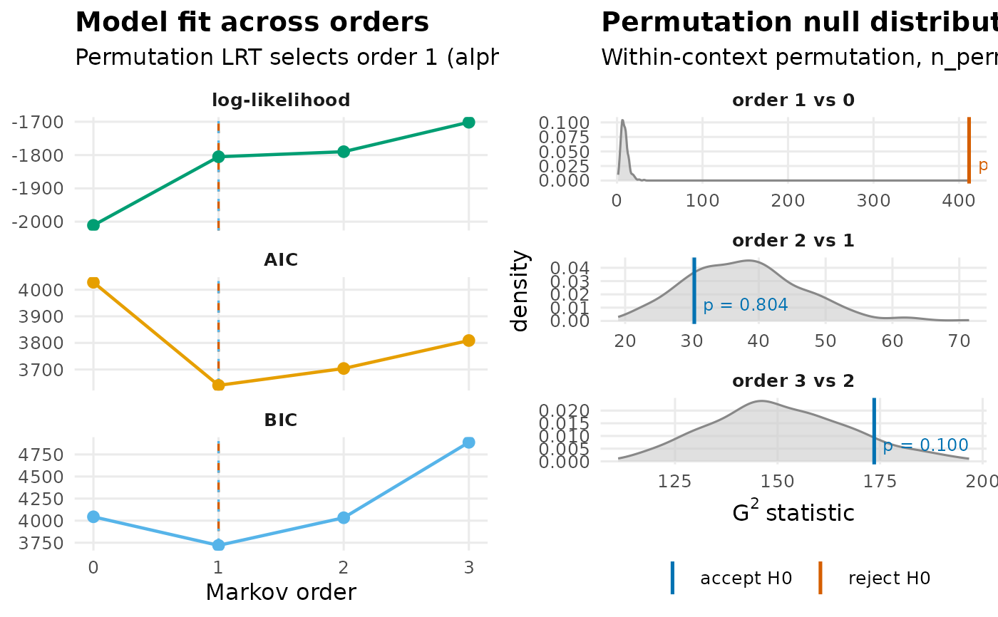
Two-panel professional visualization:
Panel A: log-likelihood, AIC, BIC across tested orders with the selected order highlighted (both the permutation-selected order and the BIC-minimizing order are marked).
Panel B: permutation null density per order with the observed \(G^2\) as a vertical marker; colored by rejection at
alpha.
Uses the Okabe-Ito colorblind-safe palette.
Examples
# Is one previous state enough to predict the next one?
res <- markov_order_test(as.data.frame(trajectories),
                         max_order = 2, n_perm = 99, seed = 1)
res
#> Markov Order Test  [within-w permutation, n_perm = 99, alpha = 0.050]
#>   131 sequences / 1865 observations / 3 states
#>
#>   Selected order  BIC: 2   AIC: 2   permutation-LRT: 2
#>
#>  order   loglik     AIC     BIC df     g2 p_permutation  p_asymptotic
#>      0 -1945.82 3895.63 3906.69 NA     NA            NA            NA
#>      1 -1636.59 3289.19 3333.43  4 618.31          0.01 1.691520e-132
#>      2 -1557.51 3167.02 3310.83 12 154.97          0.01  5.554253e-27
#>  significant
#>           NA
#>         TRUE
#>         TRUE
summary(res)
#>   order    loglik      AIC      BIC df       g2 p_permutation  p_asymptotic
#> 1     0 -1945.815 3895.630 3906.692 NA       NA            NA            NA
#> 2     1 -1636.593 3289.185 3333.434  4 618.3053          0.01 1.691520e-132
#> 3     2 -1557.511 3167.023 3310.829 12 154.9677          0.01  5.554253e-27
#>   significant
#> 1          NA
#> 2        TRUE
#> 3        TRUE
plot(res)