Grouped Transition Models: One Network per Condition

Mohammed Saqr

University of Eastern Finland

Sonsoles López-Pernas

University of Eastern Finland

Manuel J. Gómez

University of Murcia

The question

Does the same person regulate their effort differently on different kinds of day? The esm_srl study prompted 41 students up to a few times a day for momentary reports of self-regulation, motivation, and anxiety on 0-100 scales, and each report carries a day_type label: weekday or weekend. A single transition network estimated from all of it would answer how momentary effort moves between low, mid, and high on average, and in doing so would erase exactly the distinction the day-type column exists to draw.

The group argument of ts_tna() and its siblings answers the conditional question instead: one network per day type, both cut from one shared state alphabet, packaged so that Nestimate’s grouped verbs compare them directly.

library(tsn)
library(Nestimate)

data(esm_srl)

One call, one network per condition

group names a column of the data. Every level of that column becomes its own fully estimated ts_tna model. Effort has four missing values, so the incomplete rows are set aside first.

effort_rows <- subset(esm_srl, !is.na(effort))

by_day <- ts_tna(
  effort_rows,
  value = "effort",
  id = "name",
  time = "occasion",
  group = "day_type",
  labels = c("low", "mid", "high")
)

by_day
#> Group Networks (2 groups, group_col: day_type)
#> 
#>   Group    Nodes  Edges  Weights
#>   weekday  3      9      [0.098, 0.631]
#>   weekend  3      9      [0.085, 0.633]

Two day types, two networks. as.data.frame() with what = "groups" is the tidy index of how much data stands behind each one, and it is where every grouped analysis should start.

as.data.frame(by_day, what = "groups")
#>     group type sequences observations states edges
#> 1 weekday  tna       238         2033      3     9
#> 2 weekend  tna       233          783      3     9

The weekday network rests on 2,033 observations in 238 sequences, the weekend network on 783 in 233. The sequences column is the one to read closely: a sequence is cut at every change of student and at every change of day type, so a working week of roughly two reports a day forms one sequence of eight to ten observations, while a weekend forms one of three to four. The two cut rules are not the same. A change of student separates measurements that were never consecutive; a change of day type falls between two genuinely adjacent measurements, and the transition across it, from Friday evening to Saturday morning, is excluded from both networks because it belongs to neither day type. The next section shows what goes wrong without that rule.

Why not subset the data and build each model by hand?

Subsetting looks equivalent: keep the weekend rows, call ts_tna() on them, repeat for weekdays. It is not equivalent, and it fails in two distinct ways.

weekend_alone <- ts_tna(
  subset(effort_rows, day_type == "weekend"),
  value = "effort",
  id = "name",
  time = "occasion",
  labels = c("low", "mid", "high")
)

head(summary(series_networks(weekend_alone)), 3)
#>   series type observations states edges
#> 1  Amara  tna           15      3     7
#> 2    Bao  tna           22      3     8
#> 3   Cira  tna           22      3     8

First failure: the subset welds broken time back together

The hand-built model holds each student’s weekend reports as one sequence. The first student’s 15 weekend reports above span many separate weekends, yet they form a single unbroken series. Across all 41 students the 783 weekend observations become 41 sequences carrying 742 transitions. The grouped index showed the truth: those observations form 233 separate weekend runs, which contain only 783 − 233 = 550 genuine transitions. The hand-built model therefore counts 192 transitions, about a quarter of its total, between measurements that were never adjacent in time. Each one joins the end of one weekend to the start of the next across an entire intervening week, and each is a transition that never occurred.

The grouped model never counts them. A sequence is cut at every change of group, so a transition is only ever counted between genuinely consecutive measurements within one day type.

Second failure: each subset learns its own thresholds

The second failure is quieter. The default discretization = "quantile" cuts at the tertiles of whatever data it is given, so the hand-built weekend model learns cut points from weekend reports alone:

summary(
  discretize(
    subset(effort_rows, day_type == "weekend"),
    value = "effort",
    id = "name",
    time = "occasion",
    labels = c("low", "mid", "high")
  )
)
#>   state count proportion mean_value
#> 1   low   261  0.3333333   28.04603
#> 2   mid   261  0.3333333   63.07903
#> 3  high   261  0.3333333   86.32532

By construction, exactly a third of weekend reports land in each state (261 apiece), so the weekend composition can carry no information at all. The grouped model cuts the states from the pooled series before splitting, and its weekend column reports the real composition on the shared scale:

state_distribution(by_day)
#>     group state count proportion
#> 1 weekday   low   694  0.3413674
#> 2 weekday  high   676  0.3325135
#> 3 weekday   mid   663  0.3261190
#> 4 weekend   mid   268  0.3422733
#> 5 weekend  high   262  0.3346105
#> 6 weekend   low   253  0.3231162

On this panel the distortion happens to be mild, because weekday and weekend effort sit at nearly the same level (means of 58.5 and 59.2): the shared scale puts each weekend state within a percentage point or two of a third. That mildness is a property of these data, not of the method. For groups that differ in level, such as a clinical against a control cohort or a high- against a low-workload term, per-subset tertiles redefine the states inside each group, and the artifact grows with the very difference under study. The grouped model makes the safe construction the default; explicit breaks (as in vignette("nestimate-workflow", package = "tsn")) achieve the same discipline by hand.

The collection is data

Every view of the grouped model is a data frame with a leading group column. The default view is the edge list:

head(as.data.frame(by_day), 6)
#>     group from  to    weight
#> 1 weekday  low low 0.6199021
#> 2 weekday  mid low 0.2944162
#> 3 weekday high low 0.1150592
#> 4 weekday  low mid 0.2822186
#> 5 weekday  mid mid 0.4297800
#> 6 weekday high mid 0.2538071

Because both groups share one alphabet, a single edge can be read across them:

subset(as.data.frame(by_day), from == "high" & to == "mid")
#>      group from  to    weight
#> 6  weekday high mid 0.2538071
#> 15 weekend high mid 0.3419689

The probability that a high-effort report softens to mid is 0.254 on weekdays and 0.342 on weekends. This is the edge the inference section below puts to the test. what = "series" returns the per-observation table behind the networks, with the run-level sequence IDs, and summary() adds Nestimate’s network-metric panel, one column per group:

summary(by_day)
#> Network metrics by group:
#>                       metric weekday weekend
#>                   Node Count       3       3
#>                   Edge Count       9       9
#>              Network Density       1       1
#>                Mean Distance  0.2199  0.2278
#>            Mean Out-Strength       1       1
#>              SD Out-Strength 0.03206  0.1015
#>             Mean In-Strength       1       1
#>               SD In-Strength       0       0
#>              Mean Out-Degree       3       3
#>                SD Out-Degree       0       0
#>  Centralization (Out-Degree)       0       0
#>   Centralization (In-Degree)       0       0
#>                  Reciprocity       1       1

Most rows are structural constants for a full three-state network, but the standard deviation of out-strength is not: 0.032 on weekdays against 0.102 on weekends. Weekday rows spread their probability almost evenly; weekend rows are the more polarized ones.

Composition and dynamics

Composition

The state distributions above showed both day types holding close to a third of reports in each state. The mosaic view draws the transition structure itself, one panel per group, with tile area encoding transition probability:

mosaic_plot(by_day)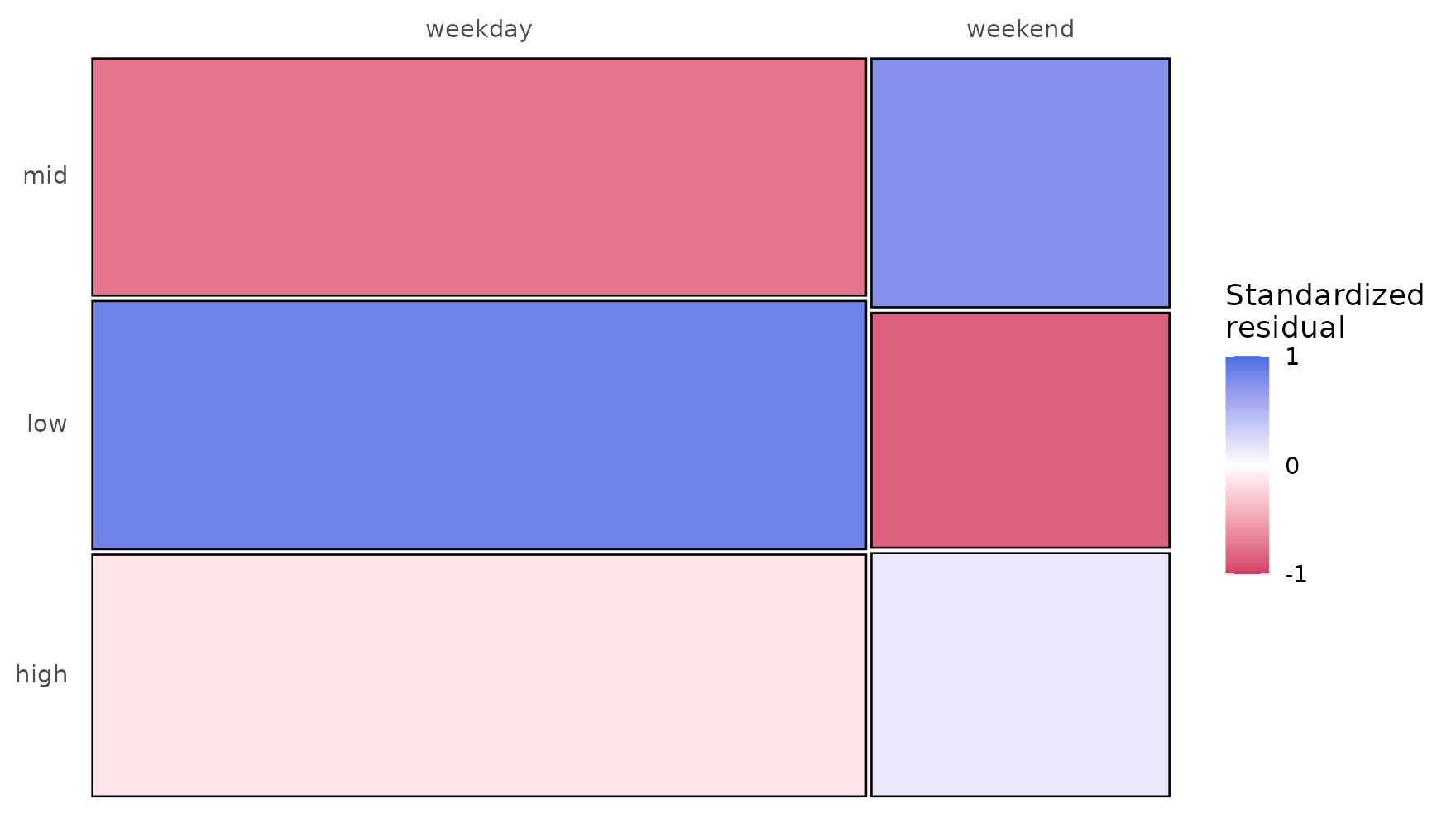

The two mosaics differ mainly at the high state: the weekend network routes more probability from high to mid (0.342 against 0.254) and retains less in high (0.534 against 0.631). This is the same softening the edge table reported, now shown as tile area rather than as a number.

Mean first passage times

passage_time() reports, per group, the expected number of steps to reach each state from each other state (Kemeny & Snell, 1976).

passage_time(by_day)
#> Mean First Passage Times -- 2 groups: weekday, weekend
#> 
#> --- weekday ---
#> Mean First Passage Times (3 states)
#> 
#>      low mid high
#> low  2.9 3.6  6.4
#> mid  4.6 3.1  5.0
#> high 5.9 3.8  3.0
#> 
#> Stationary distribution:
#>    low    mid   high 
#> 0.3483 0.3200 0.3317 
#> 
#> --- weekend ---
#> Mean First Passage Times (3 states)
#> 
#>      low mid high
#> low  2.8 3.4  6.7
#> mid  4.7 2.7  5.1
#> high 5.6 3.1  3.6
#> 
#> Stationary distribution:
#>    low    mid   high 
#> 0.3549 0.3666 0.2785

The travel times are broadly similar, since every state is reachable within three to seven steps on either day type, but the stationary distributions tilt: the weekday chain settles with 33.2% of its time in high, the weekend chain with 27.9%. Since the observed compositions are nearly identical, that tilt is carried by the dynamics, and it points at the same place the edge table did: weekends hold high effort less firmly.

Entropy and centrality

transition_entropy(by_day)
#> Transition Entropy - 2 groups: weekday, weekend
#> 
#> Entropy rate per group:
#> weekday weekend 
#>  1.3650  1.3853

Both day types run near the log2(3) = 1.585 ceiling, at 1.37 and 1.39 bits, so momentary effort is weakly predictable everywhere; neither day type is a regime of rigid habit.

day_centrality <- net_centrality(by_day)
#> centralities computed excluding loops (diagonal). Pass `loops = TRUE` to include self-transitions.

day_centrality
#> $weekday
#>      state InStrength Betweenness  Diffusion
#> low    low  0.4094755           0 0.08338405
#> mid    mid  0.5360257           2 1.00000000
#> high  high  0.3736830           0 0.00000000
#> 
#> $weekend
#>      state InStrength Betweenness Diffusion
#> low    low  0.3854634           0 0.0000000
#> mid    mid  0.6244548           2 1.0000000
#> high  high  0.3569680           0 0.6771486
#> 
#> attr(,"measures")
#> [1] "InStrength"  "Betweenness" "Diffusion"  
#> attr(,"class")
#> [1] "net_centrality_group" "list"

plot(day_centrality)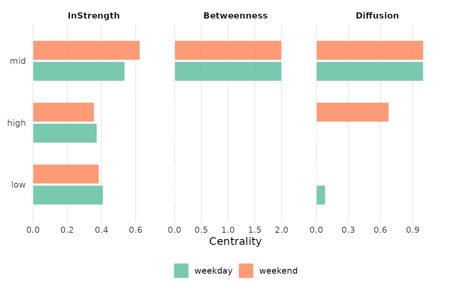

mid is the hub of both networks. It carries the highest in-strength (0.54 weekday, 0.62 weekend) and is the only state with nonzero betweenness, because movement between low and high routes through the middle of the scale. The message printed above the tables matters for any transition network: self-transitions are excluded by default, or the diagonal would drown the between-state structure.

net_edge_betweenness() runs group-wise as well, with one caveat: its result drops back to a plain netobject_group, so apply tsn’s tidy accessors before this step, not after it.

net_edge_betweenness(by_day)
#> Group Networks (2 groups)
#> 
#>   Group    Nodes  Edges  Weights
#>   weekday  3      4      [2.000, 2.000]
#>   weekend  3      4      [2.000, 2.000]

Drawing the networks

There is no single picture of a grouped model; plot() draws one selected group with the full plot.ts_tna() surface.

plot(by_day, group = "weekday", type = "network")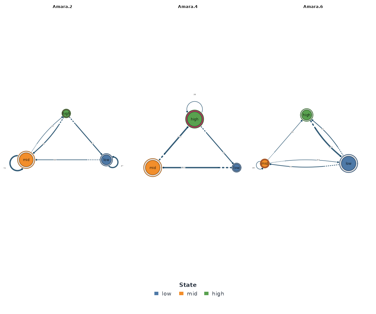

plot(by_day, group = "weekend", type = "network")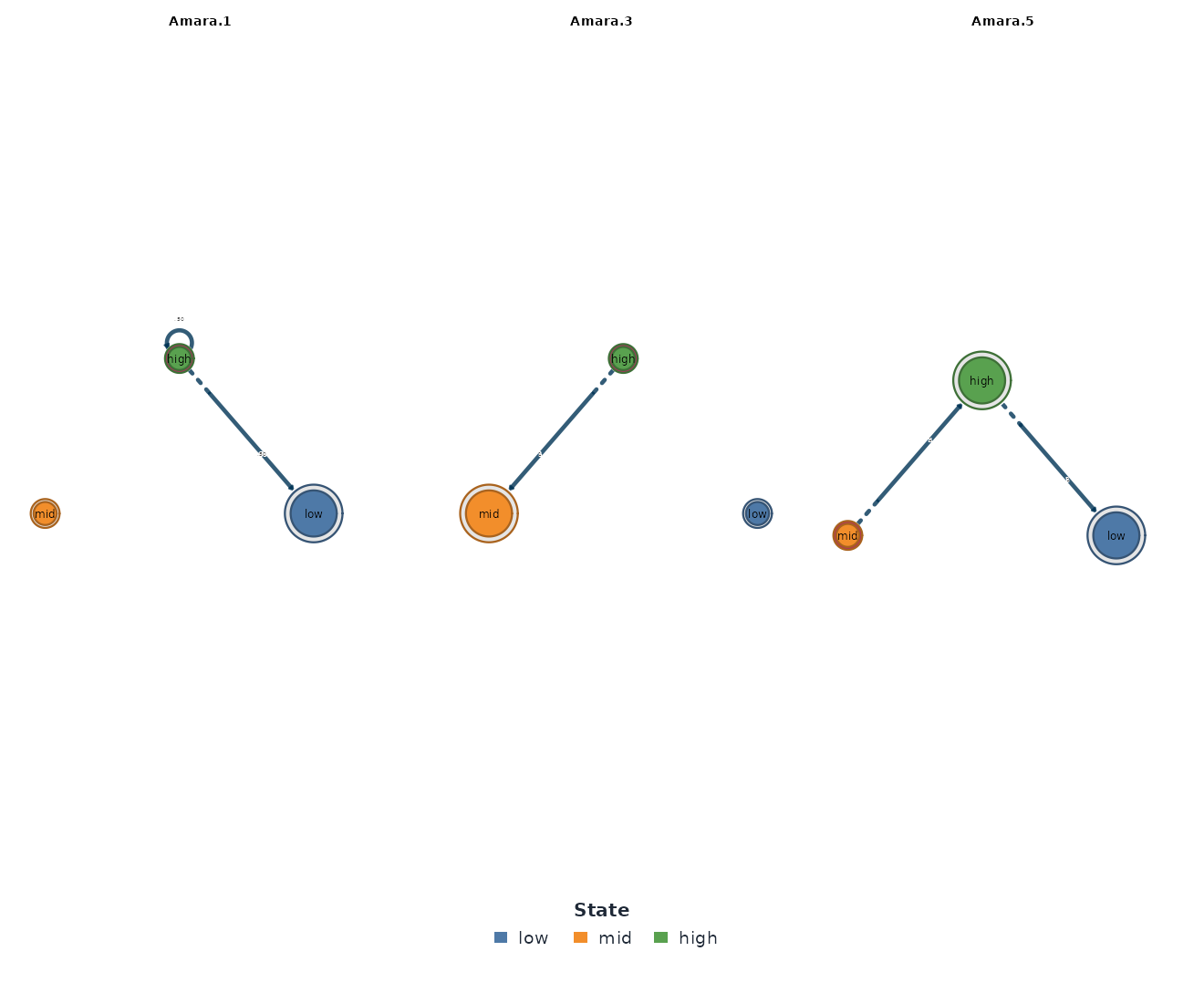

Because the two networks share one node set, the figures are directly comparable, and the difference to look for is concentrated at the high node: its self-loop is heavier on weekdays (0.631 against 0.534) and its outflow to mid heavier on weekends.

Are the differences real?

The permutation test

permutation() on a grouped model shuffles sequences between the groups to build a null distribution per edge.

day_comparison <- permutation(by_day, iter = 1000, seed = 2026)

summary(day_comparison)
#>                group from   to   weight_x   weight_y          diff  effect_size
#> 1 weekday vs weekend  low  low 0.61990212 0.63276836 -0.0128662409 -0.289921277
#> 2 weekday vs weekend  low  mid 0.28221860 0.28248588 -0.0002672786 -0.006925447
#> 3 weekday vs weekend  low high 0.09787928 0.08474576  0.0131335195  0.584487518
#> 4 weekday vs weekend  mid  low 0.29441624 0.26111111  0.0333051325  0.900900323
#> 5 weekday vs weekend  mid  mid 0.42978003 0.46666667 -0.0368866328 -0.878891544
#> 6 weekday vs weekend  mid high 0.27580372 0.27222222  0.0035815003  0.093352074
#> 7 weekday vs weekend high  low 0.11505922 0.12435233 -0.0092931099 -0.329460065
#> 8 weekday vs weekend high  mid 0.25380711 0.34196891 -0.0881618053 -2.327154276
#> 9 weekday vs weekend high high 0.63113367 0.53367876  0.0974549153  2.092734296
#>      p_value   sig
#> 1 0.77722278 FALSE
#> 2 0.99500500 FALSE
#> 3 0.56143856 FALSE
#> 4 0.38061938 FALSE
#> 5 0.37662338 FALSE
#> 6 0.92007992 FALSE
#> 7 0.77822178 FALSE
#> 8 0.02297702  TRUE
#> 9 0.04595405  TRUE

One difference holds up under the null: high -> mid (0.254 weekday, 0.342 weekend, p = 0.023). Its mirror image, the fall in high -> high retention from 0.631 on weekdays to 0.534 on weekends, sits exactly on the significance boundary (p = 0.046) and moves around 0.05 under other seeds, so it should be read as suggestive rather than established. Together they tell one coherent story: on weekends, a high-effort spell is more likely to soften into the mid range and less likely to hold. The other seven edges do not differ, so weekday and weekend self-regulation share most of their structure.

The metric panel

compare_model() condenses the pair into matrix-comparison metrics.

compare_model(by_day, i = "weekday", j = "weekend")
#> Network comparison
#> ==================
#> Summary metrics:
#>              category               metric   value
#>     Weight Deviations      Mean Abs. Diff. 0.03277
#>     Weight Deviations    Median Abs. Diff. 0.01313
#>     Weight Deviations            RMS Diff. 0.04735
#>     Weight Deviations       Max Abs. Diff. 0.09745
#>     Weight Deviations Rel. Mean Abs. Diff. 0.09832
#>     Weight Deviations             CV Ratio   1.059
#>          Correlations              Pearson  0.9657
#>          Correlations             Spearman  0.8333
#>          Correlations              Kendall  0.6667
#>          Correlations             Distance  0.9357
#>       Dissimilarities            Euclidean   0.142
#>       Dissimilarities            Manhattan   0.295
#>       Dissimilarities             Canberra  0.4608
#>       Dissimilarities          Bray-Curtis 0.04916
#>       Dissimilarities            Frobenius   0.116
#>          Similarities               Cosine  0.9922
#>          Similarities              Jaccard  0.9063
#>          Similarities                 Dice  0.9508
#>          Similarities              Overlap  0.9508
#>          Similarities                   RV  0.9744
#>  Pattern Similarities       Rank Agreement       1
#>  Pattern Similarities       Sign Agreement       1
#> 
#> Network metrics (x vs y):
#>                       metric       x      y
#>                   Node Count       3      3
#>                   Edge Count       9      9
#>              Network Density       1      1
#>                Mean Distance  0.2199 0.2278
#>            Mean Out-Strength       1      1
#>              SD Out-Strength 0.03206 0.1015
#>             Mean In-Strength       1      1
#>               SD In-Strength       0      0
#>              Mean Out-Degree       3      3
#>                SD Out-Degree       0      0
#>  Centralization (Out-Degree)       0      0
#>   Centralization (In-Degree)       0      0
#>                  Reciprocity       1      1

A Pearson correlation of 0.966 between the two weight matrices, with a maximum absolute difference of 0.097 on the high -> high retention: close networks whose one real gap is how long high effort lasts. Always name i and j, because with more than two groups there is no meaningful default pair.

Bootstrap and Bayesian certainty per group

bootstrap_network() resamples sequences within each group; certainty() reaches a similar verdict from a Dirichlet posterior, without resampling.

bootstrap_network(by_day, iter = 200, seed = 2026)
#>   Edge                   weekday   weekend 
#>   --------------------------------------------
#>   low→low               0.619     0.632   
#>   high→high             0.632     0.533   
#>   mid→mid               0.428     0.469   
#>   high→mid              0.254     0.342   
#> 
#> Grouped Bootstrap  [2 groups | 200 iterations | 95% CI]
#>   weekday               8 sig / 9 total
#>   weekend               4 sig / 9 total
#>   Shared (all groups)   4 edges

set.seed(2026)
certainty(by_day)
#>   Edge                   weekday   weekend 
#>   --------------------------------------------
#>   high→high             0.630     0.532   
#>   low→low               0.619     0.630   
#>   mid→mid               0.430     0.466   
#>   high→mid              0.254     0.342   
#>   mid→low               0.295     0.262   
#>   ... and 2 more shared significant edges
#> 
#> Grouped Bootstrap  [2 groups | NA iterations | 95% CI]
#>   weekday               9 sig / 9 total
#>   weekend               7 sig / 9 total
#>   Shared (all groups)   7 edges

The weekday network, with 2,033 observations behind it, keeps eight of nine bootstrap edges and all nine posterior-certain ones; the weekend network, with 783, keeps four and seven. Equal sequence counts (238 against 233) do not buy equal precision when the sequences differ in length: a weekend run is about a third as long as a weekday run, so the weekend estimates rest on less data. Reading the index table first is not a formality.

Is first order enough, per group?

markov_order_test() (after Anderson & Goodman, 1957) checks the Markov assumption group by group.

set.seed(2026)
markov_order_test(by_day)
#> Markov Order Test -- 2 groups: weekday, weekend
#> 
#> --- weekday ---
#> Markov Order Test  [within-w permutation, n_perm = 500, alpha = 0.050]
#>   238 sequences / 2033 observations / 3 states
#> 
#>   Selected order  BIC: 2   AIC: 3   permutation-LRT: 3
#> 
#>  order   loglik     AIC     BIC df    g2 p_permutation  p_asymptotic
#>      0 -2233.12 4470.24 4481.48 NA    NA            NA            NA
#>      1 -1963.44 3942.88 3987.82  4 539.1   0.001996008 2.336904e-115
#>      2 -1860.32 3772.65 3918.70 12 204.5   0.001996008  3.830703e-37
#>      3 -1803.75 3767.49 4216.87 36 111.7   0.001996008  1.110201e-09
#>  significant
#>           NA
#>         TRUE
#>         TRUE
#>         TRUE
#> 
#> --- weekend ---
#> Markov Order Test  [within-w permutation, n_perm = 500, alpha = 0.050]
#>   219 sequences / 769 observations / 3 states
#> 
#>   Selected order  BIC: 1   AIC: 2   permutation-LRT: 2
#> 
#>  order  loglik     AIC     BIC df     g2 p_permutation p_asymptotic significant
#>      0 -844.60 1693.21 1702.50 NA     NA            NA           NA          NA
#>      1 -768.44 1552.88 1590.04  4 149.69   0.001996008 2.367982e-31        TRUE
#>      2 -741.43 1534.85 1655.62 12  52.90   0.001996008 4.292255e-07        TRUE
#>      3 -720.22 1546.44 1792.63 26  28.57   0.630738523 3.311396e-01       FALSE

The weekday test prefers a higher order (BIC selects 2, AIC and the permutation LRT select 3): within a working week, yesterday’s effort carries information beyond today’s. The weekend test is more temperate, since BIC keeps order 1 and the LRT stops at 2, though its shorter runs give order-3 contexts little data in which to show up. Read both networks as one-step summaries, with the weekday summary the more visibly incomplete of the two.

Stability under case dropping

Two checks ask whether the results would survive a smaller sample: centrality_stability() for the centrality orderings, casedrop_reliability() for the edge weights themselves (both after Epskamp, Borsboom & Fried, 2018).

set.seed(2026)
centrality_stability(by_day, iter = 100)
#> Centrality Stability (2 networks, threshold = 0.70)
#>         InStrength OutStrength Betweenness
#> weekday        0.6         0.7         0.9
#> weekend        0.7         0.5         0.8

day_reliability <- casedrop_reliability(by_day, iter = 100, seed = 2026)

day_reliability
#> Edge-weight Case-dropping Stability (2 networks, threshold = 0.70)
#>         n_cases n_edges  CS
#> weekday     238       6 0.3
#> weekend     233       6 0.5

plot(day_reliability)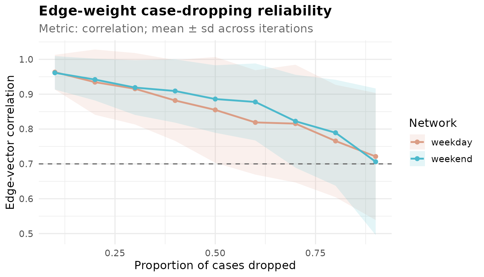

The verdicts are mixed, and the mixture is the point. The centrality orderings are serviceable (coefficients of 0.5 to 0.9), but the edge-weight CS-coefficients come back at 0.3 for weekdays and 0.5 for weekends, at or below the 0.5 bar for acceptable stability. Individual edge weights from this panel should be reported with their intervals, not as point values, and the permutation result above should carry the inferential weight. A stability check that returns an uncomfortable number has done its job.

Pruning the collection

net_prune() applies group-wise and returns the same class, so a pruned collection flows back into every verb above.

net_prune(by_day, method = "threshold", threshold = 0.3)
#> Group Networks (2 groups)
#> 
#>   Group    Nodes  Edges  Weights
#>   weekday  3      5      [0.098, 0.631]
#>   weekend  3      5      [0.085, 0.633]

Each day type keeps five of its nine edges at a 0.3 threshold. Prune after testing, not before: the high -> mid edge that carries the weekend difference sits at 0.254 on weekdays, so a premature prune would have deleted one side of the finding.

What to watch for

Four failure modes, all of which announce themselves:

• A level with almost no data. Every level of the grouping column gets a network, however little stands behind it. The groups index is the guard; read sequences and observations before edges.
• A group column that alternates too fast. Every change of group cuts a sequence, so a column that flips at almost every observation leaves runs of length one and no transitions at all. In the extreme case, a group whose observations are never adjacent, the model warns that the group’s network is empty. Day type is a well-behaved grouping variable precisely because it changes only twice a week.
• A group whose rows do not survive discretization. Temporal discretizers such as ordinal drop tail rows that cannot fill an embedding window. If that removes a group entirely, the model warns that the group was lost to discretization. A group you excluded yourself via series is not warned about, because that exclusion was your decision.
• Comparing a grouped model with a hand-subset model. The two are not estimates of the same thing, for both reasons in the section above.

When to use which

• group. The condition already exists as a column, there may be more than two levels, and the comparison itself is the point. Pooled discretization and boundary-safe sequence cutting come built in.
• Two models plus permutation(x, y). The split is not a column but a derived rule (an occasion cutoff, an external roster), and there are exactly two sides. Fix the state alphabet yourself with explicit breaks, or the comparison inherits the threshold artifact. The companion vignette vignette("nestimate-workflow", package = "tsn") runs this design on the srl panel’s course halves.
• series_networks(). The unit of comparison is the individual student (one network per person), not a condition shared across students.
• A single pooled model. No conditioning variable at all; the average dynamics are the question.

References

Anderson, T. W., & Goodman, L. A. (1957). Statistical inference about Markov chains. The Annals of Mathematical Statistics, 28(1), 89–110.

Epskamp, S., Borsboom, D., & Fried, E. I. (2018). Estimating psychological networks and their accuracy: A tutorial paper. Behavior Research Methods, 50(1), 195–212.

Kemeny, J. G., & Snell, J. L. (1976). Finite Markov Chains. Springer.