Sequence Plot (heatmap, index, or distribution)

Single entry point for three categorical-sequence visualisations.

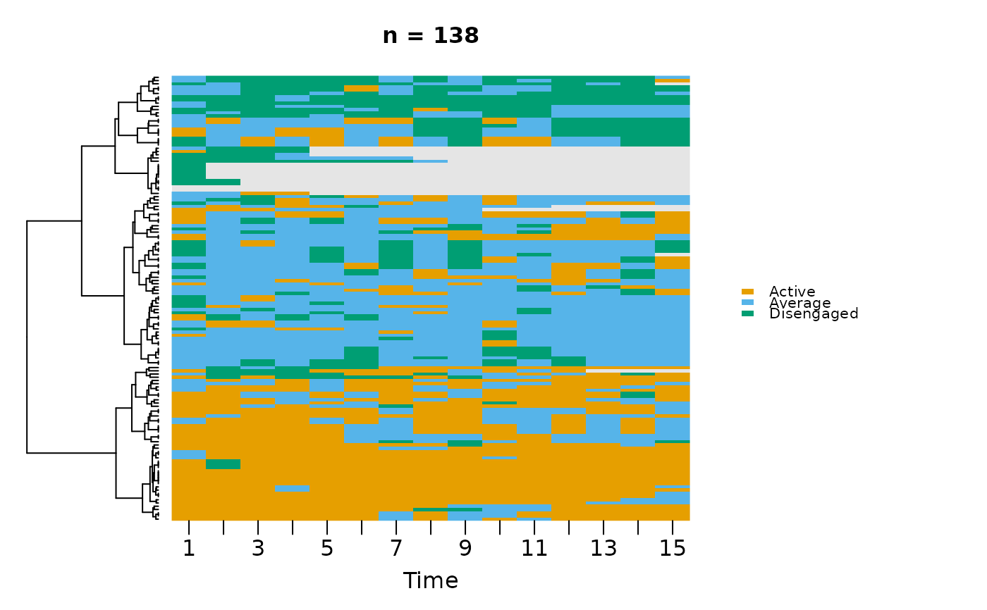
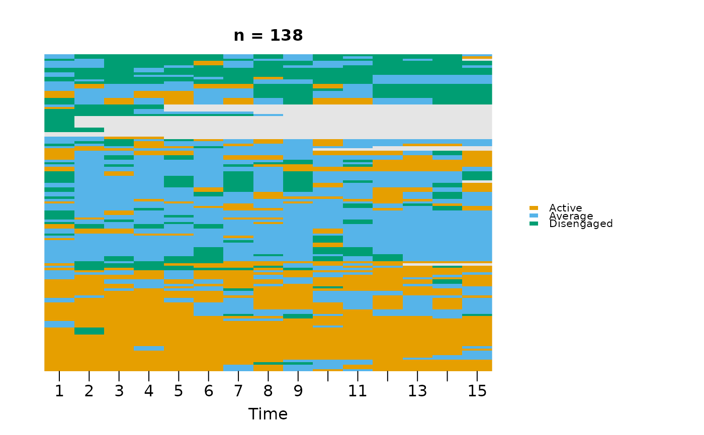
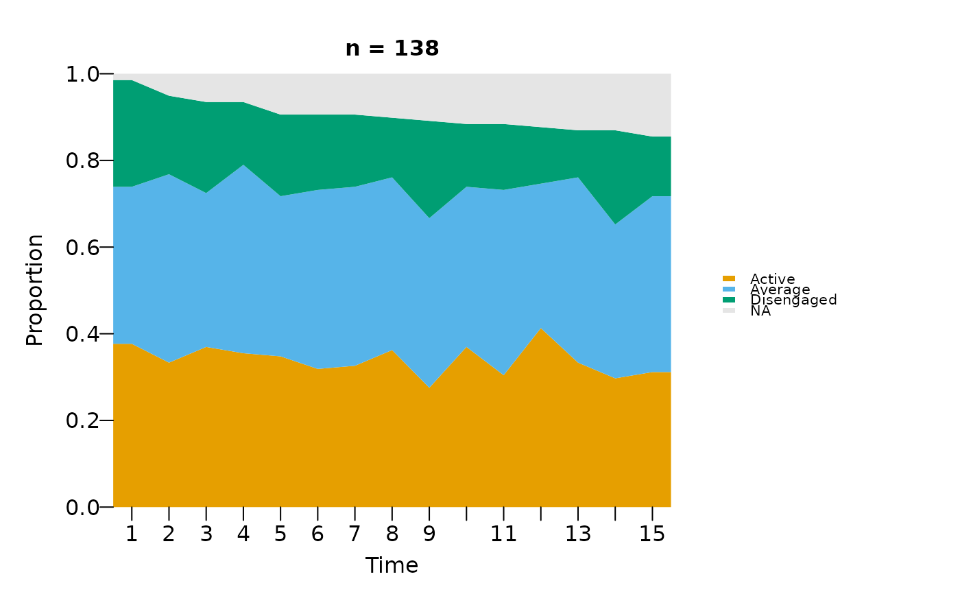
type = "heatmap" (default): dense carpet, rows reordered by sort / dendrogram (single panel).
type = "index": same data layout, but rows separated by thin gaps (no dendrogram). Supports grouping via group or a net_clustering, plus a ncol x nrow facet grid.
type = "distribution": dispatches to distribution_plot.

Usage

sequence_plot(
  x,
  type = c("heatmap", "index", "distribution"),
  sort = c("lcs", "frequency", "start", "end", "hamming", "osa", "lv", "dl", "qgram",
    "cosine", "jaccard", "jw"),
  tree = NULL,
  group = NULL,
  scale = c("proportion", "count"),
  geom = c("area", "bar"),
  na = TRUE,
  normalize = FALSE,
  trim = NULL,
  panel = c("both", "summary", "channels"),
  expand = NULL,
  combine = NULL,
  rest = c("clusters", "pooled", "none"),
  rest_label = "Other states",
  trim_clusterwise = FALSE,
  row_gap = 0,
  dendrogram_width = 1.2,
  k = NULL,
  k_color = "white",
  k_line_width = 2.5,
  state_colors = NULL,
  na_color = "grey90",
  cell_border = NA,
  frame = FALSE,
  width = NULL,
  height = NULL,
  main = NULL,
  show_n = TRUE,
  time_label = "Time",
  xlab = NULL,
  y_label = NULL,
  ylab = NULL,
  tick = NULL,
  ncol = NULL,
  nrow = NULL,
  combined = TRUE,
  legend = NULL,
  legend_size = NULL,
  legend_title = NULL,
  legend_ncol = NULL,
  legend_border = NA,
  legend_bty = "n"
)

# S3 method for class 'mcml_sequence_plot'
print(x, ...)

Arguments

x

Wide-format sequence data. Accepts:

data.frame / matrix: Rows = sequences, columns = time points.
netobject: Extracts $data.
net_clustering: From build_clusters. Uses $data, $assignments for grouping, and $distance for dendrogram.
netobject_group: From cluster_network or build_network on a clustering. Extracts data and assignments from attr(, "clustering").
net_mmm: From build_mmm. Uses $data (falling back to $models[[1]]$data) and $assignments.
tna: From the tna package. Decodes integer-encoded sequences.
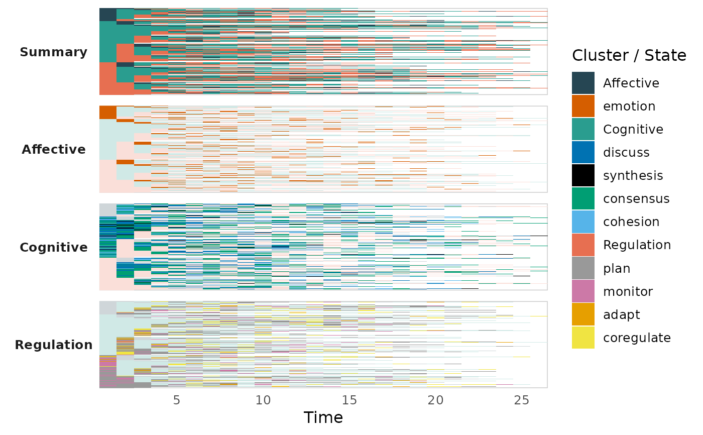
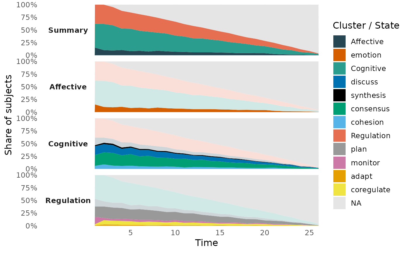
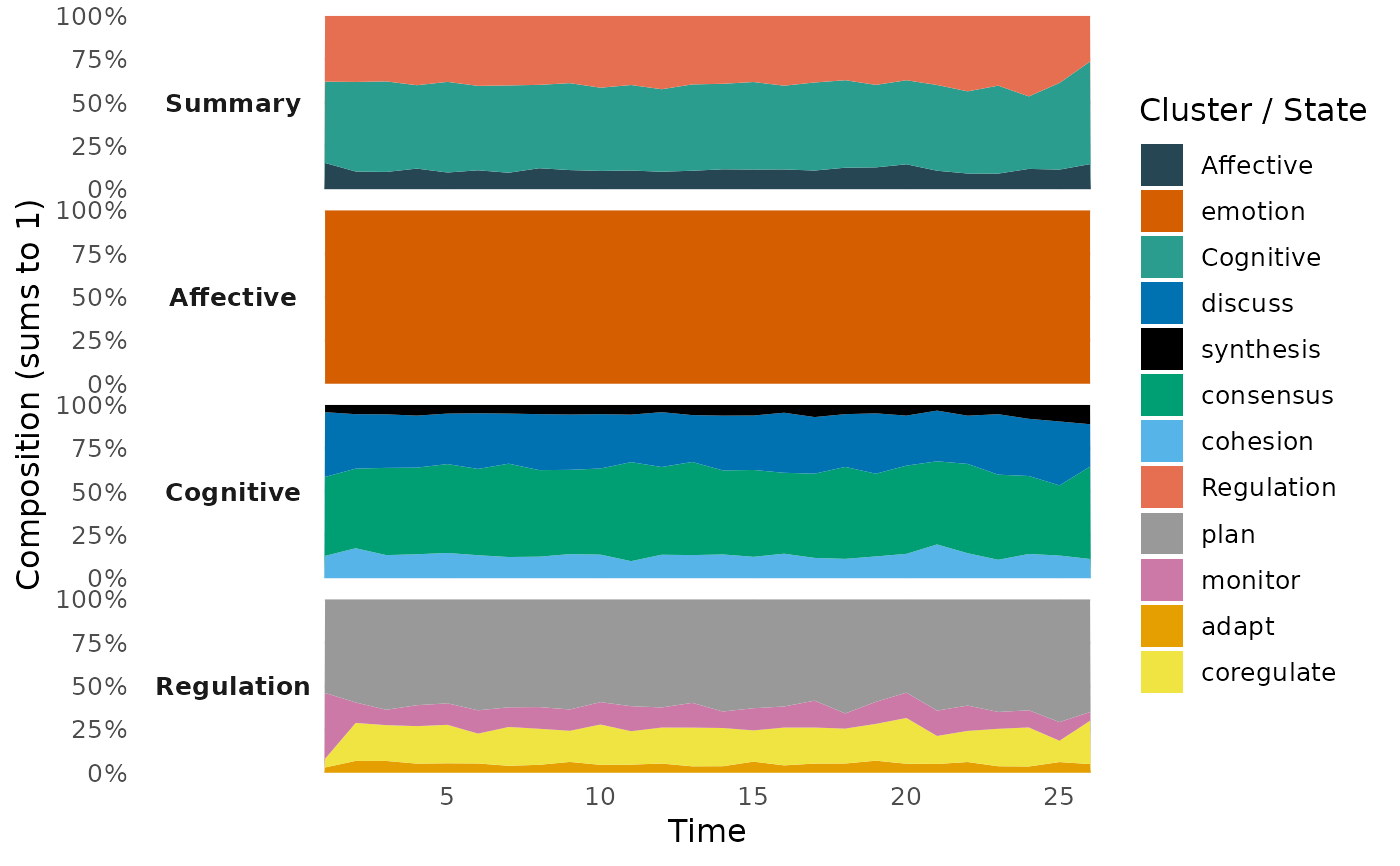
mcml: From build_mcml (built from sequences). Produces a multichannel plot: one panel per cluster plus a macro Summary panel. type = "heatmap"/"index" draw the carpet (each channel's own states solid, other clusters a faded wash); type = "distribution" draws the stacked distribution (add normalize = TRUE for a TraMineR-style seqdplot where each time point sums to 1). See the section Multichannel view of an mcml for the options that shape it, and Value for what it returns.

For the print() method: an object of class mcml_sequence_plot.

type

One of "heatmap" (default), "index", or "distribution".

sort

Row-ordering strategy for heatmap / within-panel for index. One of "lcs" (default), "frequency", "start", "end", or any build_clusters distance ("hamming", "osa", "lv", "dl", "qgram", "cosine", "jaccard", "jw").

tree

Optional hclust/dendrogram/agnes object to supply row ordering (heatmap only; overrides sort).

group

Optional grouping vector (length nrow(x)) producing one facet per group. Index/distribution only. Ignored for heatmap.

scale, geom, na

Passed to distribution_plot when type = "distribution". For an mcml (type = "distribution"), na = FALSE drops the NA (ended) band and shows every time point as shares of the sequences still running there, so each panel stacks to 100 percent (cluster panels only with rest = "clusters" or "pooled"; a time point where no sequence is running stays empty).

normalize

mcml + type = "distribution" only. When TRUE, each time point is normalised to sum to 1 within its channel (TraMineR-style seqdplot composition); when FALSE (default) the stack shows prevalence and is capped with an NA band.

trim

Optional time-axis truncation, to stop a few long sequences from stretching the plot. Applies to all three types (including the mcml multichannel view). NULL (default) plots the full width. A fraction in (0, 1) drops everything past that quantile of sequence lengths (e.g. trim = 0.95 keeps the columns covering the shortest 95% of sequences); a value >= 1 is an absolute cut (trim = 50 keeps the first 50 time points).

panel

mcml + type = "distribution" only. Which panel to draw. "both" (default) stacks the macro Summary channel and the per-cluster channels on one figure, each with its own legend; "summary" draws the macro channel alone, keyed and coloured by cluster; "channels" draws the per-cluster channels alone, keyed and coloured by state. The macro channel is keyed by cluster and the rest by state, so a cluster and a state can land on the same colour – drawing one panel avoids that and gives it a default title.

expand

For an mcml, names of clusters whose member states are shown individually in the Summary band; "all" or TRUE expands every cluster. The per-cluster channels are unaffected. Default NULL keys the Summary band by cluster.

combine

For an mcml, clusters to merge into one channel. A character vector merges one group (e.g. combine = c("Cognitive", "Affective")); a list merges several, and its names label the merged channels (default label "Cognitive + Affective"). A merged group acts as one cluster throughout the figure: one per-cluster panel holding all its states, one key in the Summary band, and one faded band in the other panels. expand is resolved after merging, so it can name the merged label. Errors on unknown clusters, a group of fewer than two, or a cluster in two groups. Default NULL draws the partition as built.

rest

For an mcml, how a cluster's panel shows the time its subjects spend in other clusters. "clusters" (default): one faded band (or wash, in the carpet) per other cluster. "pooled": all other clusters as one grey band labelled rest_label. "none": left blank, so the panel shows only its own states; in the distribution view the NA (ended) band is dropped too, and the panel's height at each time point is the share of subjects in that cluster. Ignored with normalize = TRUE, which rescales each panel to its own states. The Summary panel is unaffected.

rest_label

For an mcml, the legend text for time spent in other clusters. Default "Other states"; e.g. "Others" or "Rest of states". The pooled band (rest = "pooled") takes it as is; the per-cluster bands read "Social (Other states)". Must not equal a state or cluster name.

trim_clusterwise

Grouped type = "index" / "distribution" only, and only when trim is a fraction. FALSE (default) computes one cutoff on the pooled data and applies it to every panel, so all facets share the same width and the time axes stay aligned. TRUE crops each group to its own length quantile, so panels can end up at different widths (ragged axes). Absolute trim (>= 1) ignores this - the column is the same everywhere either way.

row_gap

Fraction of row height used as vertical gap between sequences in index plots. 0 (default) = dense like heatmap. Try 0.15 for visible separators at low row counts.

dendrogram_width

Width ratio of the dendrogram panel (heatmap).

k

Optional integer. When supplied in type = "heatmap", cuts the dendrogram into k clusters and draws thin horizontal separators between them in the carpet. Ignored when there is no dendrogram (e.g. sort = "start") or for other types.

k_color

Colour for the cluster separator lines. Default "white".

k_line_width

Line width for the cluster separators. Default 2.5.

state_colors

Colours for the fill keys. Two forms: unnamed - one colour per state, in level order (states are ordered as sort(unique(...))); named - a lookup, where only the keys you name are overridden and every other key keeps its default. Names this figure does not draw are dropped with a message naming them, so one project-wide palette can be handed to every plot and each takes the keys that apply to it.

For an mcml the named form reaches the whole figure, not just the states: a cluster name colours its Summary band, its channel strip and its faded band in the other panels, and a group merged by combine is named by its label (the list name you gave it, or "A + B"). rest_label is a key too. So state_colors = c(plan = "#0072B2", "Planning + Monitoring" = "#D55E00") recolours one state and one combined cluster and leaves the rest of the palette alone.

na_color

Colour for NA cells.

cell_border

Cell border colour. NA (default) = off.

frame

FALSE (default) draws no box - axis ticks and labels still appear. TRUE draws a box around each panel.

width, height

Optional device dimensions in inches. When supplied, opens a new graphics device via grDevices::dev.new(). In knitr chunks use the fig.width / fig.height chunk options instead.

main

Plot title.

show_n

Append "(n = N)" to the title.

time_label, xlab

X-axis label. xlab is an alias.

y_label, ylab

Y-axis label (distribution only). ylab alias.

tick

Show every Nth x-axis label. NULL = auto.

ncol, nrow

Facet grid dimensions (index + distribution). Ignored when combined = FALSE.

combined

Index and distribution types only. When TRUE (default), groups are arranged on one figure via graphics::layout(). When FALSE, each group is drawn on its own page (one full-size figure per group, with its own legend). Single-group calls (G == 1) ignore this argument. Heatmap is always single-figure.

legend

Legend position: "bottom", "right", or "none". NULL (default) resolves to "right" for every type.

legend_size

Legend text size. NULL (default) auto-scales from the device width so the legend looks proportional at 5 in vs 12 in figures (clamped to [0.65, 1.2]).

legend_title

Optional legend title.

legend_ncol

Number of legend columns.

legend_border

Swatch border colour.

legend_bty

"n" or "o".

...

In print.mcml_sequence_plot(): Ignored.

Value

An mcml input returns the multichannel figure: one panel per channel (the macro Summary and one per cluster), stacked, each with its own legend of its own clusters or states. When more than one channel is drawn this is an mcml_sequence_plot (a gtable whose print method draws it); when panel = "summary" leaves a single channel it is a plain ggplot. Every other input draws with base graphics and returns, invisibly, a list whose shape depends on type:

"heatmap": ord (integer row order actually plotted), codes (the integer-encoded, trimmed sequence matrix), palette, levels (state labels, parallel to palette), and sort_used (the ordering strategy applied, "net_clustering" when a clustering dendrogram was used).
"index": codes, palette, levels, orders (list of integer row orders, one per panel, indexing the original rows) and groups (panel labels).
"distribution": Whatever distribution_plot returns: counts, proportions, levels, palette, groups.

In print.mcml_sequence_plot(): x, invisibly. Called for the side effect of drawing it on a new page of the current graphics device.

Multichannel view of an mcml

An mcml built from sequences stores, for every cluster, the full sequence matrix with the other clusters' states blanked out. Each cluster is therefore a channel, and sequence_plot() stacks them:

Summary: The macro sequence: at every time point, the cluster each subject is in.
One panel per cluster: That cluster's own states, plus the time its subjects spend in the other clusters.

The options apply in this order, so each one sees the result of the one before:

combine merges clusters into one channel. The merged group is then one cluster throughout the figure: one panel with all its states, one Summary key, one band in the other panels. The object itself is not changed.
expand opens clusters (including a merged group, by its label) into their member states in the Summary panel only.
rest and rest_label set how a cluster's panel shows the other clusters: one faded band per cluster labelled "<cluster> (<rest_label>)" (rest = "clusters"), one grey band labelled rest_label ("pooled"), or nothing ("none").
na (distribution only) keeps the NA band of sequences that have ended (TRUE, shares of all subjects) or drops it (FALSE, shares of the subjects still running, so every panel stacks to 100 percent unless rest = "none"). normalize = TRUE instead rescales each cluster panel to its own states, which ignores rest and na.

panel draws the Summary or the cluster panels alone, and trim cuts the time axis for every panel at once.

Methods

print.mcml_sequence_plot(): Print method for the figure sequence_plot returns for an mcml with more than one channel: one panel per channel (the macro Summary and one per cluster), each with its own legend.

Examples

sequence_plot(trajectories)


# \donttest{
sequence_plot(trajectories, type = "index")

sequence_plot(trajectories, type = "distribution")


# Multichannel MCML view: one channel per cluster + a macro Summary.
fit <- build_mcml(
  group_regulation_long,
  clusters = list(Cognitive  = c("discuss", "synthesis", "consensus", "cohesion"),
                  Regulation = c("plan", "monitor", "adapt", "coregulate"),
                  Affective  = "emotion"),
  actor = "Actor", action = "Action", time = "Time")
sequence_plot(fit)                                          # multichannel carpet


# Shape the multichannel view (see the section above).
sequence_plot(fit, type = "distribution",
              combine = list(Task = c("Cognitive", "Regulation")),
              expand = "Task")                              # merge, then open


# Colour by name: one state, one cluster, one combined group. Everything
# not named keeps its default colour.
sequence_plot(fit, type = "distribution",
              combine = list(Task = c("Cognitive", "Regulation")),
              state_colors = c(Task = "#0072B2", Affective = "#D55E00",
                               emotion = "#CC79A7"))

# }