Transition Networks from Time Series: Estimation and Inference with Nestimate

Introduction

A numeric time series records the level of a quantity over time. A transition network records something different: how a system moves between a small number of qualitative states, with nodes for the states and directed edges for the probability of passing from one to the next. The two descriptions answer different questions. The series says how high a measurement was; the network says what a measurement is likely to be followed by. Recovering the second from the first takes two steps, reducing the continuous series to a sequence of states and estimating the state-to-state transitions, and then a third that is easy to skip: deciding what such a model may legitimately claim.

The tsn package performs the first two steps in a single call and hands the result to Nestimate, which supplies the third. ts_tna() discretizes a series, estimates the transition network, and returns a native Nestimate model, so Nestimate’s descriptive and inferential verbs apply to it with no conversion step in between. This vignette follows one analysis through the whole path: building the model, reading its structure, and, where the data support it, testing that structure with bootstrap confidence intervals, centrality stability, a Markov-order test, and a permutation comparison of two periods.

The distinction between description and inference organizes everything below. Descriptive summaries such as centralities, state distributions, entropy, and pruning ask what a fitted network looks like, and a network fitted to a single series answers them. Inference asks how far the estimate would move under a different sample, and a single series is a single sample: there is nothing to resample. The dividing line is the unit of analysis, and knowing where it falls is what keeps a transition model from being read for more than it can support.

library(tsn)
library(Nestimate)

data(motivation)
data(steps)

From measurements to a model

ts_tna() takes a data frame and the name of one numeric column, cuts that column into states, and estimates the transition network in one call. Here it runs on the first 200 observations of the pleasure rating from the motivation study, an intensive-longitudinal record of momentary experience.

pleasure <- head(motivation, 200)

model <- ts_tna(
  pleasure,
  series = "pleasure",
  labels = c("low", "mid", "high")
)

model
#> Transition Network (relative probabilities) [directed]
#>   Weights: [0.278, 0.417]  |  mean: 0.333
#> 
#>   Weight matrix:
#>          low   mid  high
#>   low  0.403 0.313 0.284
#>   mid  0.278 0.417 0.306
#>   high 0.333 0.367 0.300 
#> 
#>   Initial probabilities:
#>   high          1.000  ████████████████████████████████████████
#>   low           0.000  
#>   mid           0.000

The printed object is the complete model: a row-stochastic weight matrix whose entry (i, j) is the probability of moving to state j given that the system is currently in state i, together with the initial-state distribution. Each row sums to one because from any state the process must go somewhere.

The bridge: this object is a Nestimate model

Everything that follows rests on one property of the returned object.

class(model)
#> [1] "ts_tna"          "netobject"       "cograph_network"

ts_tna() does not return a private structure that must be converted before Nestimate can read it. It returns an object that inherits from netobject, Nestimate’s core network class, and Nestimate’s verbs dispatch on that class directly. There is no export step and no adapter call between the model and the tests applied to it, which is what lets a single analysis move from construction to inference without leaving the object behind.

Four constructors, one interface

The same discretized sequence supports four definitions of an edge, and the four constructors take identical arguments and return the same class. ts_tna() gives relative frequencies, so an edge is the conditional probability of the next state. ts_ftna() gives the raw transition counts behind those probabilities. ts_atna() applies attention weighting, and ts_cna() counts undirected co-occurrence rather than directed movement. Changing the edge definition means changing only the constructor.

ts_ftna(pleasure, series = "pleasure", labels = c("low", "mid", "high"))
#> Transition Network (frequency counts) [directed]
#>   Weights: [18.000, 30.000]  |  mean: 22.111
#> 
#>   Weight matrix:
#>        low mid high
#>   low   27  21   19
#>   mid   20  30   22
#>   high  20  22   18 
#> 
#>   Initial probabilities:
#>   high          1.000  ████████████████████████████████████████
#>   low           0.000  
#>   mid           0.000

The remainder of the vignette uses ts_tna(), because the inferential tests are written for probabilities.

One series, and what it can support

Asking a single-series model for a bootstrap returns a warning rather than a result:

A network with one long sequence is not recommended and can’t be validated using bootstrap and other confirmatory testings.

The warning is correct. A bootstrap resamples sequences to estimate how far a quantity would move under a different sample of them; one series is one sequence, so there is nothing to resample and no sampling distribution to form. The permutation and stability tests rest on the same logic.

This is a statement about the unit of analysis, not a dead end. A long series contains many transitions; what it lacks is a way to group them into units that can be resampled. The segment argument supplies that unit by cutting the series into shorter blocks, each treated as its own sequence. This is the block bootstrap, and tsn provides its two standard forms.

The series below is one participant’s 299 daily step counts. Two features of the call matter before the segmenting itself. States are cut at 5,000 and 10,000 steps with discretization = "threshold" rather than at the default tertiles, so the states mean the same thing outside this sample; the next section returns to why that matters. And segmentation is applied after discretization, so every block inherits the same cut points and no block is ever discretized against itself.

walkers <- subset(steps, !is.na(steps))
one_walker <- subset(walkers, id == 193)

whole <- ts_tna(
  one_walker,
  value = "steps",
  time = "day",
  discretization = "threshold",
  breaks = c(5000, 10000),
  labels = c("sedentary", "moderate", "active")
)

Partitioning cuts the 299 observations into consecutive, non-overlapping blocks. At segment = 10 there are thirty of them.

blocks <- ts_tna(
  one_walker,
  value = "steps",
  time = "day",
  segment = 10,
  discretization = "threshold",
  breaks = c(5000, 10000),
  labels = c("sedentary", "moderate", "active")
)

bootstrap_network(blocks, iter = 500, seed = 2024)
#>   Edge                   Mean     95% CI          p
#>   -----------------------------------------------
#>   active → moderate    0.558  [0.457, 0.653]  ** 
#>   moderate → moderate   0.437  [0.336, 0.525]  *  
#> 
#> Bootstrap Network  [Transition Network (relative) | directed]
#>   Iterations : 500  |  Nodes : 3
#>   Edges      : 2 significant / 9 total
#>   CI         : 95%  |  Inference: stability  |  CR [0.75, 1.25]

Thirty sequences, and the bootstrap now runs. Partitioning is not free: every cut destroys the transition that straddles it, so thirty blocks cost roughly thirty of the 298 transitions and the estimate shifts slightly.

Sliding the window instead of partitioning keeps all of them. At segment = 2, overlap = TRUE the blocks are the consecutive lag-1 pairs, so every transition appears exactly once and the network is identical to the unsegmented one.

lag_one <- ts_tna(
  one_walker,
  value = "steps",
  time = "day",
  segment = 2,
  overlap = TRUE,
  discretization = "threshold",
  breaks = c(5000, 10000),
  labels = c("sedentary", "moderate", "active")
)

all.equal(as.matrix(lag_one), as.matrix(whole))
#> [1] TRUE

bootstrap_network(lag_one, iter = 500, seed = 2024)
#>   Edge                   Mean     95% CI          p
#>   -----------------------------------------------
#>   active → moderate    0.559  [0.459, 0.659]  ** 
#>   moderate → moderate   0.426  [0.344, 0.504]  ** 
#>   moderate → active    0.359  [0.285, 0.439]  *  
#> 
#> Bootstrap Network  [Transition Network (relative) | directed]
#>   Iterations : 500  |  Nodes : 3
#>   Edges      : 3 significant / 9 total
#>   CI         : 95%  |  Inference: stability  |  CR [0.75, 1.25]

The two schemes trade precision against independence. Sliding blocks preserve the point estimate exactly, yield the most units, and tend to give narrower intervals: a mean width of 0.18 here against 0.21 for the partitioned blocks, narrow enough to call a third edge significant where partitioning calls two. The tendency is not a guarantee, since two of the nine edges come out wider. And the narrowness carries a cost. Overlapping blocks share observations, so they are not independent, and resampling lag-1 pairs assumes exactly the first-order Markov property the model itself assumes. That is the assumption the Markov-order test below rejects for these data, which makes those intervals optimistic.

Partitioned blocks are the more conservative choice. A block preserves whatever dependence exists inside it, so structure beyond one lag survives resampling, at the price of the boundary transitions lost to the cuts. Blocks of 10 to 30 retain 90% to 97% of the transitions, which is usually the right trade; blocks of 2 retain only half and are better avoided.

None of this manufactures information. Segmenting a single series asks how stable one person’s own dynamics are, and says nothing about anyone else. A claim about people in general needs people in general, so the rest of the vignette uses all 151 of them.

Choosing states that mean something

The default discretization = "quantile" cuts at the tertiles, forcing each of the three states to hold a third of the observations, so the state sizes carry no information, by construction. That is why every model built from the steps data uses fixed thresholds of 5,000 and 10,000 steps instead. Fixed breaks make the states interpretable outside the sample, and they give every model one shared alphabet, which is what makes the period comparison below legitimate. (The grouped pleasure model at the end keeps the quantile default; grouping pools the series before cutting it, so its groups share an alphabet without breaks being named.)

walk_model <- ts_tna(
  walkers,
  value = "steps",
  id = "id",
  time = "day",
  discretization = "threshold",
  breaks = c(5000, 10000),
  labels = c("sedentary", "moderate", "active")
)

walk_model
#> Transition Network (relative probabilities) [directed]
#>   Weights: [0.062, 0.619]  |  mean: 0.333
#> 
#>   Weight matrix:
#>             sedentary moderate active
#>   sedentary     0.353    0.445  0.202
#>   moderate      0.154    0.501  0.345
#>   active        0.062    0.320  0.619 
#> 
#>   Initial probabilities:
#>   active        0.576  ████████████████████████████████████████
#>   moderate      0.311  ██████████████████████
#>   sedentary     0.113  ████████

The states now mean something outside the data, the same cut points apply to every comparison made later, and the state distribution is worth reading.

state_distribution(walk_model)
#>   group     state count proportion
#> 1   all    active 13921  0.4484425
#> 2   all  moderate 12776  0.4115582
#> 3   all sedentary  4346  0.1399994

Every state is strongly self-preferring, and an active day is the most persistent of all at 0.62: activity, once reached, tends to continue. Step counts show marked day-to-day inertia.

One network per person

The pooled model estimates a single network across everyone. series_networks() splits it into one complete model per participant, each rebuilt on the same alphabet so node sets stay aligned and comparable.

per_person <- series_networks(walk_model)

head(summary(per_person))
#>   series type observations states edges
#> 1     35  tna          295      3     6
#> 2     37  tna          278      3     9
#> 3     47  tna          297      3     9
#> 4     57  tna          239      3     9
#> 5     58  tna          176      3     9
#> 6     70  tna          257      3     9

Each row indexes a full ts_tna model that prints and plots on its own: the models are the list elements, and this is the tidy index over them. Because the cut points are fixed step counts rather than sample quantiles, a participant’s personal network describes their own activity, not their rank within the sample.

Describing the model

Centrality

net_centrality(walk_model)
#> centralities computed excluding loops (diagonal). Pass `loops = TRUE` to include self-transitions.
#>               state InStrength Betweenness Diffusion
#> sedentary sedentary  0.2152510           0 1.0000000
#> moderate   moderate  0.7650336           1 0.4116171
#> active       active  0.5470912           0 0.0000000

The message notes that centralities exclude self-transitions by default, which matters for a transition network: the diagonal is usually the largest entry, so a state can be highly persistent while receiving little traffic from elsewhere. Excluding the diagonal measures how central a state is to movement between states rather than to staying put. Passing loops = TRUE includes it.

How much of the sequence is structure, and how much is noise

transition_entropy(walk_model)
#> Transition Entropy (3 states, bits; ceiling = 1.585)
#> 
#>                           raw            normalised
#>   Entropy rate    h(P)  = 1.346 bits    0.849
#>   Stationary    H(pi)  = 1.444 bits    0.911
#>   Redundancy   H(pi)-h = 0.098 bits    0.068
#> 
#> Normalised: h(P) and H(pi) are raw / log_2(n_states) (0 = deterministic, 1 = uniform);
#>   redundancy is the relative redundancy (H(pi) - h(P)) / H(pi), not raw / log_2(n_states).

The entropy rate is normalized against log2(n_states), so 0 is a perfectly deterministic process and 1 means every next state is equally likely from wherever the process currently sits. A value of 1 requires more than an uninformative current state: a lopsided but state-independent process still scores well below it. Cut at the tertiles, these same step counts score 0.93; cut at 5,000 and 10,000 they score 0.85. The cut points are not cosmetic: they decide how much structure is left to find.

Pruning

Not every edge deserves a place in the picture. net_prune() returns a model of the same class with weak edges removed, so its result flows straight back into any verb above.

net_prune(walk_model, method = "threshold", threshold = 0.3)
#> Transition Network (relative probabilities) [directed]
#>   Weights: [0.320, 0.619]  |  mean: 0.430
#> 
#>   Weight matrix:
#>             sedentary moderate active
#>   sedentary     0.353    0.445  0.000
#>   moderate      0.000    0.501  0.345
#>   active        0.000    0.320  0.619 
#> 
#>   Initial probabilities:
#>   active        0.576  ████████████████████████████████████████
#>   moderate      0.311  ██████████████████████
#>   sedentary     0.113  ████████

Three edges fall below the threshold: every route into sedentary from a higher state, together with the direct leap from sedentary to active. What survives says that a sedentary day is harder to fall into than to climb out of. The sedentary -> moderate edge is a strong 0.445, while nothing descends into sedentary above 0.3.

Prune after testing rather than before, however. A threshold ranks edges by size, and size is not the same as interest: a small but reliably estimated edge can matter more than a large but uncertain one.

Bootstrap: which edges survive resampling?

bootstrap_network() resamples the sequences with replacement, re-estimates the network on each resample, and reports a confidence interval for every edge.

boot <- bootstrap_network(walk_model, iter = 200, seed = 2024)

boot
#>   Edge                   Mean     95% CI          p
#>   -----------------------------------------------
#>   active → active      0.618  [0.585, 0.648]  ** 
#>   moderate → moderate   0.500  [0.478, 0.523]  ** 
#>   sedentary → moderate   0.444  [0.419, 0.469]  ** 
#>   sedentary → sedentary   0.353  [0.323, 0.386]  ** 
#>   moderate → active    0.346  [0.318, 0.373]  ** 
#>   ... and 4 more significant edges
#> 
#> Bootstrap Network  [Transition Network (relative) | directed]
#>   Iterations : 200  |  Nodes : 3
#>   Edges      : 9 significant / 9 total
#>   CI         : 95%  |  Inference: stability  |  CR [0.75, 1.25]

summary() returns the tidy, one-row-per-edge table.

summary(boot)
#>        from        to     weight       mean          sd     p_value  sig
#> 1 sedentary sedentary 0.35281837 0.35345581 0.016363187 0.004975124 TRUE
#> 2 sedentary  moderate 0.44514034 0.44378997 0.012517516 0.004975124 TRUE
#> 3 sedentary    active 0.20204129 0.20275421 0.012723224 0.004975124 TRUE
#> 4  moderate sedentary 0.15365259 0.15382362 0.008219952 0.004975124 TRUE
#> 5  moderate  moderate 0.50129748 0.50036003 0.011436886 0.004975124 TRUE
#> 6  moderate    active 0.34504993 0.34581635 0.014524197 0.004975124 TRUE
#> 7    active sedentary 0.06159838 0.06212676 0.005251614 0.014925373 TRUE
#> 8    active  moderate 0.31989325 0.31996300 0.011000596 0.004975124 TRUE
#> 9    active    active 0.61850837 0.61791024 0.014531904 0.004975124 TRUE
#>     ci_lower  ci_upper   cr_lower   cr_upper
#> 1 0.32318763 0.3856584 0.26461378 0.44102296
#> 2 0.41903064 0.4688517 0.33385525 0.55642542
#> 3 0.17664549 0.2244967 0.15153097 0.25255161
#> 4 0.13841919 0.1697292 0.11523944 0.19206574
#> 5 0.47778672 0.5230883 0.37597311 0.62662184
#> 6 0.31847498 0.3727507 0.25878745 0.43131242
#> 7 0.05314263 0.0738917 0.04619879 0.07699798
#> 8 0.29783560 0.3433023 0.23991994 0.39986656
#> 9 0.58489465 0.6482990 0.46388128 0.77313546

With 151 sequences behind it, every edge is estimated precisely and all nine survive resampling. Confidence intervals a few hundredths wide are what a large sample buys, and they are the ground on which the descriptive reading above can be reported rather than merely observed.

Stability: would the same states rank first in a smaller study?

centrality_stability() repeatedly drops a proportion of the sequences, re-computes the centralities, and reports the largest proportion that can be dropped while the ordering still tracks the original, a correlation-stability coefficient.

centrality_stability(walk_model, iter = 100)
#> Centrality Stability (100 iterations, threshold = 0.7)
#>   Drop proportions: 0.1, 0.2, 0.3, 0.4, 0.5, 0.6, 0.7, 0.8, 0.9
#> 
#>   CS-coefficients:
#>     InStrength       0.90
#>     OutStrength      0.90
#>     Betweenness      0.90

All three coefficients reach 0.90, against conventional bars of 0.5 for acceptable and 0.7 for excellent. That measures how stable the ordering is under resampling; it does not speak to whether the ordering is substantively meaningful, only to whether a smaller study would have recovered it.

Markov order: is a first-order model enough?

Every transition network here assumes the Markov property, that the next state depends on the current one and nothing earlier. That assumption is testable, by comparing the fit of models of increasing order.

markov_order_test(walk_model)
#> Markov Order Test  [within-w permutation, n_perm = 500, alpha = 0.050]
#>   151 sequences / 31043 observations / 3 states
#> 
#>   Selected order  BIC: 3   AIC: 3   permutation-LRT: 3
#> 
#>  order    loglik      AIC      BIC df      g2 p_permutation  p_asymptotic
#>      0 -31051.63 62107.27 62123.95 NA      NA            NA            NA
#>      1 -28961.91 57939.82 58006.57  4 4179.40   0.001996008  0.000000e+00
#>      2 -28209.20 56470.40 56687.32 12 1505.37   0.001996008 2.624960e-315
#>      3 -27901.81 55963.62 56631.07 36  614.68   0.001996008 1.933327e-106
#>  significant
#>           NA
#>         TRUE
#>         TRUE
#>         TRUE

The test disagrees with the first-order model. AIC, BIC, and the permutation likelihood-ratio test all prefer a higher order, meaning yesterday carries information about tomorrow beyond what today already conveys. This does not invalidate the first-order network, but it bounds the claim: the network is a summary of one-step behaviour, not a full description of the process.

The natural follow-up is a higher-order network.

build_hon(walk_model, max_order = 2)
#> Higher-Order Network (HON)
#>   Nodes:        3 (3 first-order states)
#>   Edges:        9
#>   Max order:    1 (requested 2)
#>   Min freq:     1
#>   Trajectories: 151

The higher-order construction keeps every node at order 1: it finds no individual context that shifts the next-step distribution enough to justify splitting the node. The two criteria disagree because they ask different questions. The likelihood test detects aggregate improvement pooled across all sequences, while the higher-order rule applies a stricter, per-node test. Both results are real, and both are worth reporting: there is higher-order structure in aggregate, but not localized in any single state.

Comparing two periods

The tests so far describe one network. permutation() compares two, shuffling the group labels to build a null distribution for every edge. The steps series runs from April 2019 to March 2020; splitting at the start of November contrasts the warmer months with the colder ones. The two spans are unequal in length, roughly six and a half months against four.

Both models are built with the same fixed breaks, which matters more than it appears: had each period been discretized on its own quantiles, the two networks would rest on different cut points, and any difference between them could reflect the thresholds rather than behaviour.

cutoff <- as.Date("2019-11-01")

early <- ts_tna(
  subset(walkers, as.Date(day) < cutoff),
  value = "steps",
  id = "id",
  time = "day",
  discretization = "threshold",
  breaks = c(5000, 10000),
  labels = c("sedentary", "moderate", "active")
)

late <- ts_tna(
  subset(walkers, as.Date(day) >= cutoff),
  value = "steps",
  id = "id",
  time = "day",
  discretization = "threshold",
  breaks = c(5000, 10000),
  labels = c("sedentary", "moderate", "active")
)

comparison <- permutation(early, late, iter = 2000, seed = 2024)

comparison
#> Permutation Test:Transition Network (relative probabilities) [directed]
#>   Iterations: 2000  |  Alpha: 0.05
#>   Nodes: 3  |  Edges tested: 9  |  Significant: 0

summary(comparison)
#>        from        to   weight_x   weight_y         diff effect_size    p_value
#> 1 sedentary sedentary 0.34985280 0.35525154 -0.005398748 -0.18420352 0.86406797
#> 2 sedentary  moderate 0.44602552 0.44395410  0.002071411  0.08267605 0.93753123
#> 3 sedentary    active 0.20412169 0.20079435  0.003327337  0.15848152 0.88655672
#> 4  moderate sedentary 0.14430829 0.16225831 -0.017950026 -1.26222133 0.20589705
#> 5  moderate  moderate 0.50048371 0.50224285 -0.001759131 -0.09494720 0.91554223
#> 6  moderate    active 0.35520800 0.33549884  0.019709158  0.87706971 0.38030985
#> 7    active sedentary 0.05810102 0.06593238 -0.007831364 -0.93700923 0.35282359
#> 8    active  moderate 0.30333977 0.33761664 -0.034276870 -1.78233216 0.07196402
#> 9    active    active 0.63855921 0.59645097  0.042108234  1.75491892 0.07946027
#>     sig
#> 1 FALSE
#> 2 FALSE
#> 3 FALSE
#> 4 FALSE
#> 5 FALSE
#> 6 FALSE
#> 7 FALSE
#> 8 FALSE
#> 9 FALSE

None of the nine edge comparisons reaches significance; the smallest p-value is 0.07. The estimates are not identical, but no difference survives the permutation null. That is a more informative result than a scattering of small p-values would have been, because the two periods differ in how much people walked in the first place:

state_distribution(early)
#>   group     state count proportion
#> 1   all    active  7328  0.4689620
#> 2   all  moderate  6253  0.4001664
#> 3   all sedentary  2045  0.1308716

state_distribution(late)
#>   group     state count proportion
#> 1   all    active  6593  0.4276448
#> 2   all  moderate  6523  0.4231044
#> 3   all sedentary  2301  0.1492508

Active days fall from 46.9% before November to 42.8% after it, and sedentary days rise. The seasonal shift is therefore plain in the composition of the states while no comparison of the transitions between them reaches significance. The estimated sedentary-to-moderate probability, for instance, is 0.446 before November and 0.444 after, with a permutation p-value of 0.94.

Two cautions bound how far that carries. Failing to reject nine tests is not the same as showing the dynamics are identical, and the two models do not rest on quite the same people: 140 participants contribute before November and 149 after, with 138 in both.

That distinction is the reason to build a transition network at all. A comparison of means or of state proportions finds the seasonal difference and stops there; the transition model asks a further question of the same population, whether the dynamics moved with the season, and finds no evidence that they did.

More than two groups: one model per context

Building two models by hand is manageable when there are two. When the variable that separates the groups is already a column in the data, the group argument builds one network per level in a single call, and it scales past two, which the pairwise form does not.

The motivation study records where each measurement was taken in task_context_type, so the pleasure ratings can be split by context.

by_context <- ts_tna(
  motivation,
  series = "pleasure",
  group = "task_context_type",
  labels = c("low", "mid", "high")
)

by_context
#> Group Networks (4 groups, group_col: task_context_type)
#> 
#>   Group     Nodes  Edges  Weights
#>   Home      3      9      [0.040, 0.762]
#>   Other     3      1      [1.000, 1.000]
#>   Personal  3      9      [0.065, 0.664]
#>   Work      3      9      [0.156, 0.518]

Two things happen here that would be tedious to arrange by hand. The states are cut from the pooled series before the split, so all four networks rest on one set of thresholds and share a node set, the same discipline the fixed breaks enforced earlier, applied automatically. And the result is a Nestimate netobject_group, so the compatible grouped verbs take it directly: net_prune(), state_distribution(), net_centrality(), compare_model(), permutation(), mosaic_plot(), and their neighbours. Not every verb applies: those needing a precision matrix or a clustering attribute reject a transition model, and there is no grouped plot() method, so networks are plotted one at a time.

as.data.frame() gives the tidy view of how much data stands behind each network:

as.data.frame(by_context, what = "groups")
#>      group type sequences observations states edges
#> 1     Home  tna       832         1324      3     9
#> 2    Other  tna         2            3      3     1
#> 3 Personal  tna       822         1309      3     9
#> 4     Work  tna       976         2235      3     9

The sequence counts repay a second look: Home has 1,324 observations but 832 sequences. That is not padding. A run is cut at every change of series and at every change of group, and the two cuts are not the same. A change of series separates measurements that were never consecutive; a change of context falls between two genuinely adjacent measurements, and the transition across it is excluded from both networks because it belongs to neither context. This study alternates context from one measurement to the next (4,871 observations form 2,632 contiguous runs), so each unbroken stretch within a context becomes its own sequence, and a pair of measurements separated by an intervening visit to a different context is never counted as a transition, because it never was one.

That rule costs nothing when a group is constant within a series, which is the usual case for a condition or a cohort: each series then contributes one sequence and keeps its own ID.

state_distribution(by_context)
#>       group state count proportion
#> 1      Home   low   827 0.62462236
#> 2      Home   mid   409 0.30891239
#> 3      Home  high    88 0.06646526
#> 4     Other  high     1 0.33333333
#> 5     Other   low     1 0.33333333
#> 6     Other   mid     1 0.33333333
#> 7  Personal  high   597 0.45607334
#> 8  Personal   mid   459 0.35064935
#> 9  Personal   low   253 0.19327731
#> 10     Work  high   938 0.41968680
#> 11     Work   mid   749 0.33512304
#> 12     Work   low   548 0.24519016

The contexts are not alike. Pleasure is low on 62.5% of measurements taken at home and high on only 6.6% of them; personal time reverses that ordering: high on 45.6%, low on 19.3%. Work sits between the two on all three states. A mosaic plot shows the same contrast in the transition structure at a glance, one panel per context:

mosaic_plot(by_con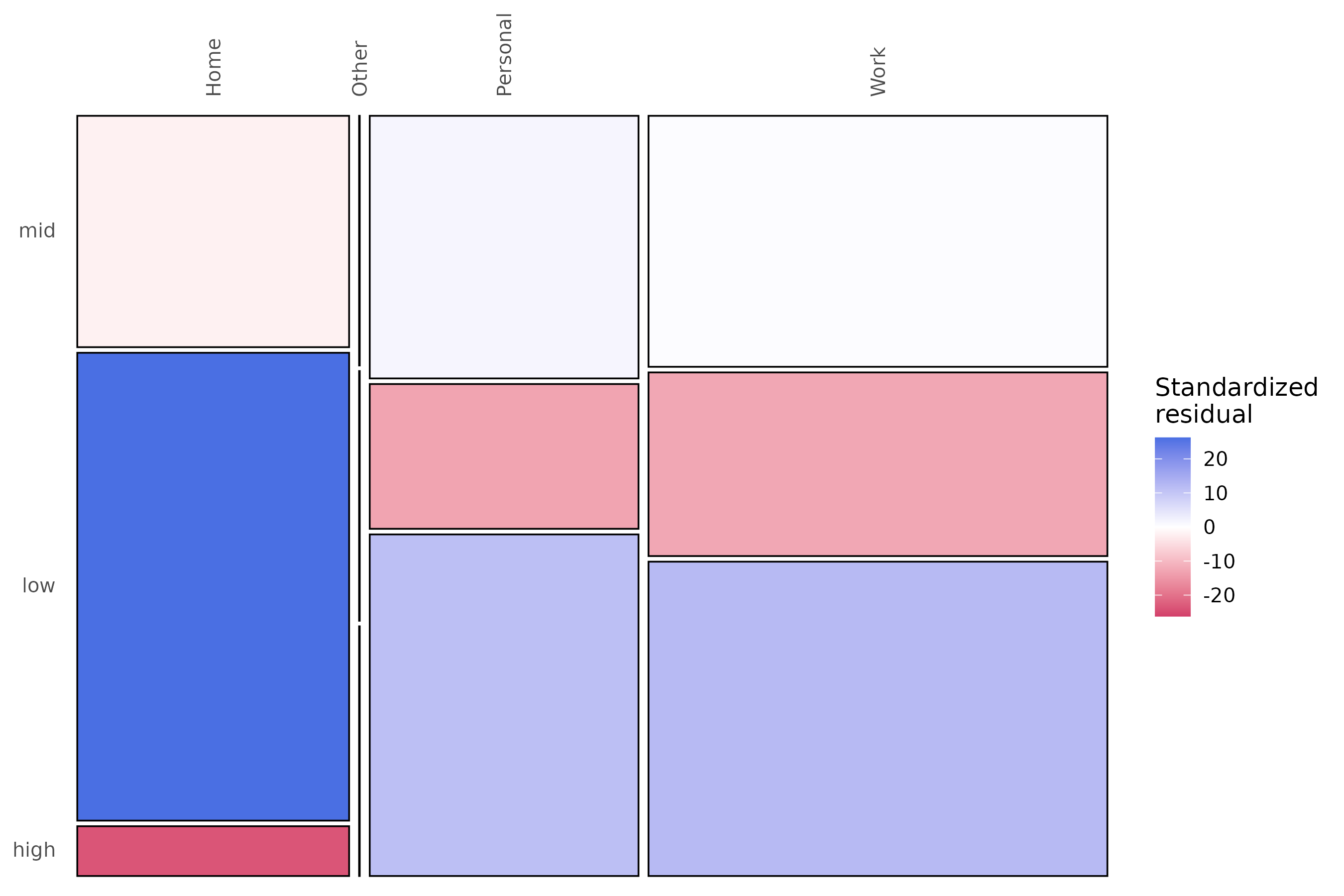text)

Mosaic panels of the four context-specific transition networks, in which tile area encodes transition probability from each current state to each next state, showing the home context concentrated in the low-to-low cell and personal time in the high-to-high cell.

Tile area encodes the transition probability from a current state (rows) to a next state (columns). The home panel is dominated by its low-to-low cell and the personal panel by its high-to-high cell, so the difference in level between the contexts reappears as a difference in persistence: wherever pleasure tends to be, it tends to stay.

Because every network shares an alphabet, two of them can be set side by side and selected by name:

compare_model(by_context, i = "Home", j = "Work")
#> Network comparison
#> ==================
#> Summary metrics:
#>              category               metric   value
#>     Weight Deviations      Mean Abs. Diff.  0.2318
#>     Weight Deviations    Median Abs. Diff.  0.2503
#>     Weight Deviations            RMS Diff.  0.2581
#>     Weight Deviations       Max Abs. Diff.  0.3699
#>     Weight Deviations Rel. Mean Abs. Diff.  0.6953
#>     Weight Deviations             CV Ratio   2.268
#>          Correlations              Pearson -0.2137
#>          Correlations             Spearman -0.2167
#>          Correlations              Kendall -0.1111
#>          Correlations             Distance  0.2513
#>       Dissimilarities            Euclidean  0.7743
#>       Dissimilarities            Manhattan   2.086
#>       Dissimilarities             Canberra   3.477
#>       Dissimilarities          Bray-Curtis  0.3477
#>       Dissimilarities            Frobenius  0.6322
#>          Similarities               Cosine  0.7693
#>          Similarities              Jaccard  0.4841
#>          Similarities                 Dice  0.6523
#>          Similarities              Overlap  0.6523
#>          Similarities                   RV  0.6594
#>  Pattern Similarities       Rank Agreement  0.8333
#>  Pattern Similarities       Sign Agreement       1
#> 
#> Network metrics (x vs y):
#>                       metric      x      y
#>                   Node Count      3      3
#>                   Edge Count      9      9
#>              Network Density      1      1
#>                Mean Distance 0.2697 0.2882
#>            Mean Out-Strength      1      1
#>              SD Out-Strength 0.7008 0.2058
#>             Mean In-Strength      1      1
#>               SD In-Strength      0      0
#>              Mean Out-Degree      3      3
#>                SD Out-Degree      0      0
#>  Centralization (Out-Degree)      0      0
#>   Centralization (In-Degree)      0      0
#>                  Reciprocity      1      1

Pruning applies group-wise and returns a grouped model, so the collection can be carried through a workflow without being taken apart:

net_prune(by_context, method = "threshold", threshold = 0.3)
#> Group Networks (4 groups)
#> 
#>   Group     Nodes  Edges  Weights
#>   Home      3      6      [0.148, 0.762]
#>   Other     3      1      [1.000, 1.000]
#>   Personal  3      6      [0.286, 0.664]
#>   Work      3      6      [0.315, 0.518]

The index table states one caution plainly rather than hiding it: Other holds three observations and two sequences. It is a level of the column, so it gets a network, but a network estimated from a single transition is not a result. Read the sequences and observations columns before reading the edges.

Plotting a single model

A grouped model has no plot() method, but any single network does, including the pooled step model. The plot draws the three states as nodes and the transition probabilities as directed edges, with self-loops for persistence.

plot(walk_model)

Transition network of daily step-count states, with sedentary, moderate, and active nodes joined by directed edges whose thickness reflects transition probability and self-loops that mark each state's persistence.

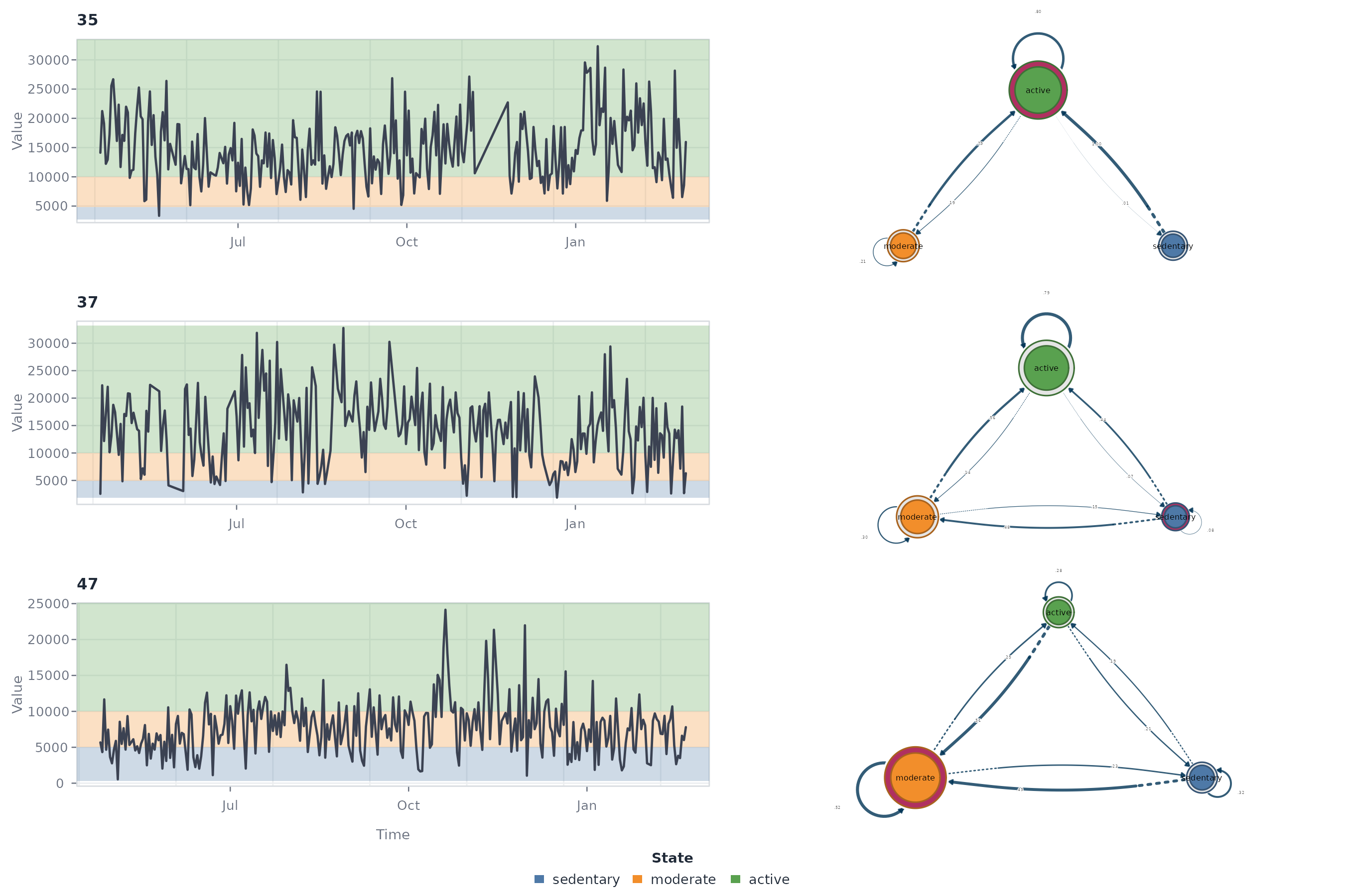
The heavy self-loops confirm what the state distribution reported numerically: each state mostly returns to itself, and movement between states is the smaller part of the process. The plotting vignette covers the plot types and their arguments in full.

Where the line falls

Everything descriptive in this vignette, from centralities, state distributions, entropy, and pruning to per-participant splits and the grouped models, runs on a model built from a single series. Everything inferential, meaning the bootstrap, stability, the Markov-order test, and the permutation test, requires many sequences, because resampling and permutation both treat the sequence as the unit of analysis.

Three practices follow. Build with id from the start if you intend to test anything, so the sequences exist when a test asks for them. Fix your breaks before you compare anything, or pass group and let the pooled discretization fix them for you, so a difference between networks is a difference in behaviour and not in thresholds. And when a comparison rests on few sequences, say so: the sequences column exists to be read.

Mohammed Saqr

Sonsoles López-Pernas

Manuel J. Gómez