Transition Entropy of a Markov Chain

Computes per-state branching entropy, stationary entropy, and the chain-level entropy rate of a Markov transition process. The entropy rate \(H = -\sum_i \pi_i \sum_j P_{ij} \log_b P_{ij}\) (with \(\pi\) the stationary distribution from the eigendecomposition of \(P^\top\) at \(\lambda = 1\)) is the Shannon-McMillan-Breiman per-step uncertainty of trajectories - the canonical information-theoretic summary of a transition matrix, introduced to behavioral research as gaze transition entropy by Krejtz et al. (2015) and tracked in real time as mobile transition matrix entropy by Krejtz et al. (2025). The normalized fields (*_norm, division by \(\log_b n\)) are the scale-free variants those papers report.

Usage

transition_entropy(x, base = 2, normalize = TRUE)

# S3 method for class 'net_transition_entropy'
print(x, digits = 3, ...)

# S3 method for class 'net_transition_entropy_group'
print(x, ...)

# S3 method for class 'net_transition_entropy'
summary(object, ...)

# S3 method for class 'summary.net_transition_entropy'
print(x, digits = 3, ...)

# S3 method for class 'net_transition_entropy'
plot(x, title = "Transition Entropy", fill = "#0072B2", ...)

Arguments

x: A netobject, cograph_network, tna object, row-stochastic numeric transition matrix, or a wide sequence data.frame (rows = actors, columns = time-steps; a relative transition network is built automatically). Group dispatch on netobject_group. For the print() and plot() methods: an object of class net_transition_entropy or net_transition_entropy_group (or its summary()).
base: Numeric. Logarithm base. 2 (default) for bits, exp(1) for nats, 10 for hartleys.
normalize: Logical. If TRUE (default), rows that do not sum to 1 are normalised automatically (with a warning).
digits: Integer. Digits to round numeric output. Default 3.
...: In plot.net_transition_entropy(), print.net_transition_entropy(), print.summary.net_transition_entropy() and summary.net_transition_entropy(): Ignored. In print.net_transition_entropy_group(): Forwarded to print.net_transition_entropy.
object: For the summary() method: an object of class net_transition_entropy.
title: Character. Plot title.
fill: Character. Bar fill colour. Default Okabe-Ito blue.

Value

An object of class "net_transition_entropy" with:

row_entropy: Named numeric vector, length \(n\). Per-state branching entropy \(H(P_{i\cdot}) = -\sum_j P_{ij} \log P_{ij}\).
row_entropy_norm: Named numeric vector. row_entropy divided by the ceiling \(\log_b n\) (in \([0, 1]\); all zeros when \(n = 1\)).
stationary: Named numeric vector. Stationary distribution \(\pi\).
stationary_entropy: Scalar. \(H(\pi) = -\sum_i \pi_i \log \pi_i\) - the entropy of \(\pi\) treated as an i.i.d. distribution. Upper bound on the entropy rate.
stationary_entropy_norm: Scalar. stationary_entropy divided by the ceiling \(\log_b n\).
entropy_rate: Scalar. \(h(P) = \sum_i \pi_i H(P_{i\cdot})\) - the Shannon-McMillan-Breiman entropy rate.
entropy_rate_norm: Scalar. entropy_rate divided by the ceiling \(\log_b n\).
redundancy: Scalar. \(H(\pi) - h(P)\), the entropy deficit attributable to serial dependence; zero for an i.i.d. chain (rows of \(P\) all equal \(\pi\)).
redundancy_norm: Scalar. The relative redundancy \((H(\pi) - h(P)) / H(\pi)\) (the fraction of the stationary entropy removed by order-1 memory), not redundancy divided by \(\log_b n\); 0 when \(H(\pi) = 0\).
max_entropy: Scalar. The normalising ceiling \(\log_b n\).
base: Logarithm base used.
states: Character vector of state names.

For a netobject_group the result is a "net_transition_entropy_group": a named list holding one such object per group.

In print.net_transition_entropy(), print.net_transition_entropy_group() and print.summary.net_transition_entropy(): x invisibly.

In summary.net_transition_entropy(): A summary.net_transition_entropy containing

table: tidy per-state data.frame, sorted by contribution_pct descending
chain: tidy chain-level data.frame with raw and normalised \(h(P)\), \(H(\pi)\), redundancy, and ceiling
base: logarithm base used

In plot.net_transition_entropy(): A ggplot object.

Details

Convention \(0 \log 0 := 0\) is applied, so absorbing or deterministic rows contribute zero per-row entropy. The chain need not be irreducible; \(\pi\) is computed from the eigendecomposition of \(P^\top\) as elsewhere in the package. For non-ergodic chains the returned \(\pi\) is one stationary distribution among many - interpret with the help of chain_structure.

The relation \(h(P) \leq H(\pi)\) holds with equality iff successive states are independent. The deficit \(H(\pi) - h(P)\) is reported as redundancy - a measure of how much memory the chain has at order 1.

Methods

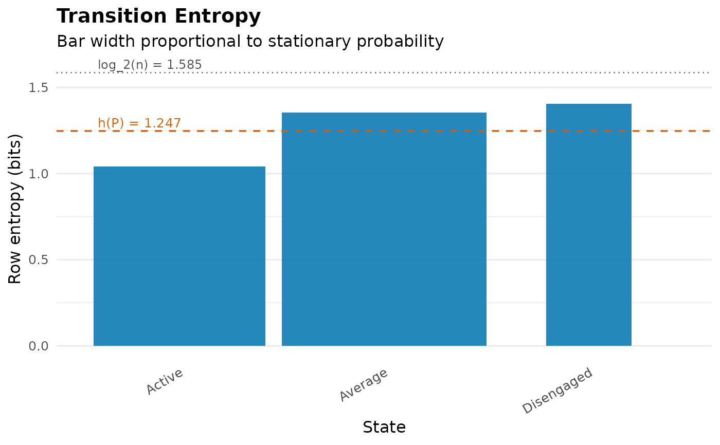
plot.net_transition_entropy(): Bar chart of per-state row entropy with overlaid horizontal lines at the entropy rate \(h(P)\) (chain-level summary) and the maximum row entropy \(\log_b n\) (uniform branching). Bar widths are proportional to the stationary probability so the visual area sums to the entropy rate.
summary.net_transition_entropy(): Returns a tidy per-state contribution table sorted by share of the chain-level entropy rate (largest first), so the dominant contributors to \(h(P)\) are visible at a glance. Each row contains the stationary mass, the raw and normalised row entropy, the additive contribution \(\pi_i H(P_{i\cdot})\), and that contribution as a percentage of \(h(P)\).

References

Cover, T.M. & Thomas, J.A. (2006). Elements of Information Theory, 2nd ed., chapter 4. Wiley.

Krejtz, K., Duchowski, A., Szmidt, T., Krejtz, I., Gonzalez Perilli, F., Pires, A., Vilaro, A., & Villalobos, N. (2015). Gaze transition entropy. ACM Transactions on Applied Perception, 13(1), 4:1-4:20. doi:10.1145/2834121

Krejtz, K., Hughes, C.J., Stasiak, I., Duchowski, A., & Krejtz, I. (2025). Real-time mobile transition matrix entropy based on eye and head movements. Proceedings of ETRA '25. doi:10.1145/3715669.3723128

Shannon, C.E. (1948). A mathematical theory of communication. Bell System Technical Journal, 27, 379-423.

Examples

net <- build_network(as.data.frame(trajectories), method = "relative")
te  <- transition_entropy(net)
print(te)
#> Transition Entropy (3 states, bits; ceiling = 1.585)
#> 
#>                           raw            normalised
#>   Entropy rate    h(P)  = 1.247 bits    0.787
#>   Stationary    H(pi)  = 1.501 bits    0.947
#>   Redundancy   H(pi)-h = 0.255 bits    0.170
#> 
#> Normalised: h(P) and H(pi) are raw / log_2(n_states) (0 = deterministic, 1 = uniform);
#>   redundancy is the relative redundancy (H(pi) - h(P)) / H(pi), not raw / log_2(n_states).
summary(te)
#> Transition Entropy Summary (bits)
#> 
#> Per-state contribution to h(P):
#>       state stationary row_entropy row_entropy_norm contribution
#>     Average      0.443       1.354            0.855        0.600
#>      Active      0.372       1.040            0.656        0.387
#>  Disengaged      0.185       1.403            0.885        0.260
#>  contribution_pct
#>              48.1
#>              31.0
#>              20.8
#> 
#> Chain-level summary:
#>               quantity   raw normalised
#>      entropy_rate h(P) 1.247      0.787
#>       stationary H(pi) 1.501      0.947
#>  redundancy H(pi)-h(P) 0.255      0.170
#>       ceiling log_2(n) 1.585      1.000
#> 
#> Normalised: row entropy, h(P) and H(pi) are raw / log_2(n_states), in [0, 1];
#>   redundancy is the relative redundancy (H(pi) - h(P)) / H(pi).
plot(te)