
Two-variable mosaic analysis (chi-square test + flat mosaic)
Source:R/mosaic_analysis.R
mosaic_analysis.RdAnalyses the association between two categorical columns of a data.frame.
Builds the contingency table, drops sparse categories below
min_count, runs a Pearson chi-square test (or Fisher's exact test),
computes Cramer's V with a df-adjusted effect-size label, and draws a flat
ggplot2 mosaic whose tile area encodes counts and whose fill encodes the
standardized Pearson residual (Nestimate diverging palette). All tabular
output is a tidy one-row-per-cell data.frame.
Usage
mosaic_analysis(
  data,
  var1,
  var2,
  min_count = 10L,
  test = c("chisq", "fisher"),
  percentage_base = c("total", "row", "column"),
  tile_label = c("count", "percent", "residual", "category", "none"),
  title = "",
  ...
)

# S3 method for class 'mosaic_analysis'
plot(x, ...)

# S3 method for class 'mosaic_analysis'
print(x, ...)

# S3 method for class 'mosaic_analysis'
summary(object, ...)
Arguments
- data
A data.frame containing the two variables.
- var1
Character. Name of the first variable (mosaic columns).
- var2
Character. Name of the second variable (stacked within columns).
- min_count
Integer. Minimum marginal count for a category to be kept. Categories of either variable below this are dropped before testing. Default 10.
- test
Character.
"chisq"(default) Pearson chi-square, or"fisher"Fisher's exact test (simulated p-value). Cramer's V and the residual fill are always derived from the chi-square statistic.- percentage_base
Character. Base for the
"percent"tile label and thepctcolumn:"total"(default),"row"(withinvar1), or"column"(withinvar2).- tile_label
Character. What to print inside each tile:
"count"(default),"percent","residual","category"(var2level), or"none".- title
Character. Plot title. Default
"".- ...
Further flat-mosaic styling arguments passed to the renderer (e.g.
col_label_side,row_label_side,legend_position,legend_size,label_size,palette). Tile fill uses the ColorBrewer RdBu ramp by default (override withpalette). Column labels auto-rotate to vertical when there are more than 6 columns; passcol_label_angleto force an angle. Inplot.mosaic_analysis(): Styling overrides forwarded to the flat renderer. Inprint.mosaic_analysis()andsummary.mosaic_analysis(): Ignored.- x
For the
plot()andprint()methods: an object of classmosaic_analysis.- object
For the
summary()method: an object of classmosaic_analysis.
Value
An object of class "mosaic_analysis": a list with
- plot
The flat mosaic
ggplotobject.- counts
Tidy data.frame, one row per (var1, var2) cell, with
observed,expected,residual(standardized), andpct(onpercentage_base).- stats
One-row data.frame:
test,statistic,df,p_value,cramers_v,effect_size,n.- test
The raw
htestobject.- cramers_v, effect_size
Effect size value and label.
- table
The filtered contingency
table.- removed
List of dropped
var1/var2categories.- n_original, n_filtered
Row counts before/after filtering.
- vars
Named character vector
c(var1 = , var2 = ).- plot_parts, plot_args
The residual matrix, table, and styling arguments retained so
plot()can re-render without re-testing.
Use print() for the test summary and summary() for the tidy
per-cell table.
In plot.mosaic_analysis(): The re-rendered flat mosaic ggplot object, invisibly; the plot is drawn on the active device as a side effect.
In print.mosaic_analysis(): x, invisibly.
In summary.mosaic_analysis(): The tidy per-cell data.frame: one row per (var1, var2) cell, with the two variable columns (named after var1 / var2) plus observed, expected, residual and pct. The one-row test summary is attached as the "stats" attribute.
Methods
plot.mosaic_analysis(): Re-renders the flat mosaic from the stored contingency table and residuals, so styling can be changed without re-running the test. Any flat-mosaic styling argument (tile_label,pct_base,col_label_side,legend_size, ...) may be overridden via....
See also
mosaic_plot for the network/table mosaic (which also
accepts style = "flat").
Examples
data(group_regulation_long, package = "Nestimate")
res <- mosaic_analysis(group_regulation_long, "Course", "Action",
min_count = 20)
res
#> Mosaic analysis: Course x Action
#> N = 27533 (filtered from 27533); table 3 x 9
#> Chi-square: X2 = 233.560, df = 16, p = 1.199e-40
#> Cramer's V = 0.065 (negligible)
head(summary(res))
#> Course Action observed expected residual pct
#> 1 A adapt 140 249.303 -9.430 0.51
#> 2 B adapt 261 193.688 6.059 0.95
#> 3 C adapt 153 111.009 4.502 0.56
#> 4 A cohesion 923 827.560 4.631 3.35
#> 5 B cohesion 590 642.945 -2.680 2.14
#> 6 C cohesion 326 368.495 -2.563 1.18
# \donttest{
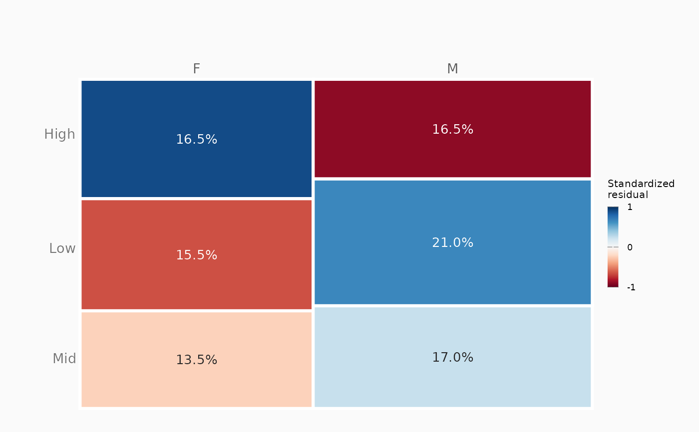
plot(res, tile_label = "percent")
 # }
# }