Diagnoses where a chain's order-1 Markov assumption fails by comparing, for each order-k context \((s_1, \ldots, s_{k-1})\), the empirical next-state distribution \(P(s_k \mid s_1, \ldots, s_{k-1})\) against the order-1 prediction \(P(s_k \mid s_{k-1})\) that uses only the most recent state. Returns a tidy per-context table sorted by Kullback-Leibler divergence so the analyst can see exactly which histories carry extra predictive information.
Usage
path_dependence(x, order = 2L, min_count = 5L, base = 2)

# S3 method for class 'net_path_dependence'
print(x, top = 10L, digits = 3L, ...)

# S3 method for class 'net_path_dependence'
summary(object, ...)

# S3 method for class 'summary.net_path_dependence'
print(x, digits = 3L, ...)

# S3 method for class 'net_path_dependence'
plot(x, top = 15L, title = NULL, ...)
Arguments
- x
A wide sequence data.frame / matrix (rows = actors, columns = time-steps), or a
netobjectthat carries the source data. For theprint()andplot()methods: an object of classnet_path_dependence(or itssummary()).- order
Integer. Order of the conditioning context.
order = 2(default) compares 2-step memory against 1-step;order = 3compares 3-step memory; etc. Must be a whole number; a non-integer value is an error rather than being silently truncated.- min_count
Integer. Drop contexts seen fewer than this many times. Default 5. Very small samples produce noisy KL estimates.
- base
Numeric. Logarithm base for entropy and KL. Default 2 (bits).
- top
In
print.net_path_dependence(): Integer. Number of top contexts to show. Default 10. Inplot.net_path_dependence(): Integer. Number of contexts to show (top by KL). Default 15.- digits
Integer. Digits to round numeric output. Default 3.
- ...
In
plot.net_path_dependence(),print.net_path_dependence(),print.summary.net_path_dependence()andsummary.net_path_dependence(): Ignored.- object
For the
summary()method: an object of classnet_path_dependence.- title
Character or
NULL. Plot title. DefaultNULL, which builds "Path dependence: order k vs order 1" from the fitted order.
Value
An object of class "net_path_dependence" with
- contexts
tidy data.frame, one row per order-k context, sorted by KL descending. Columns:
context(e.g. "A -> B"),n(count),H_order1(entropy of \(P(\cdot \mid s_{k-1})\)),H_orderk(entropy of \(P(\cdot \mid \mathrm{context})\)),H_drop(=H_order1-H_orderk),KL(= \(D_{KL}(P_k \| P_1)\)),top_o1(most likely next state under order-1),top_ok(most likely next state under order-k),flips(logical: did the most likely next state change?).- chain
list with chain-level summaries:
KL_weighted(count-weighted mean KL across contexts),H_drop_weighted(count-weighted mean entropy drop),n_contexts,n_flips(contexts where the most-likely next state changed).- order
integer
- base
numeric
- min_count
integer
- states
character vector
In print.net_path_dependence() and print.summary.net_path_dependence(): x invisibly.
In summary.net_path_dependence(): A summary.net_path_dependence with the full sorted table and chain-level summaries.
In plot.net_path_dependence(): A ggplot object.
Details
For each context \(c = (s_1, \ldots, s_{k-1})\) occurring at least
min_count times, the function computes:
the empirical conditional \(P_k(\cdot \mid c)\) from k-gram counts;
the order-1 prediction \(P_1(\cdot \mid s_{k-1})\) from the most recent state alone (the bigram-marginal estimator);
the entropy drop \(H(P_1) - H(P_k)\) - bits of uncertainty removed by extending memory by one step in this specific context;
the Kullback-Leibler divergence \(D_{KL}(P_k \,\|\, P_1)\) - bits of "surprise" if you used the order-1 model when the order-k model is true.
KL = 0 means longer history adds no information for that context.
H_drop > 0 means longer history sharpens the prediction;
H_drop < 0 indicates the order-k context happens to spread
probability across more outcomes than order-1 alone (small-sample noise
or genuine context-induced uncertainty - inspect n).
Contexts where flips = TRUE are the substantively interesting
ones: the longer history changes the modal prediction, not just its
confidence.
Pair this with markov_order_test (which decides whether
order-k is needed globally) to see the chain-level decision broken
down per context.
Methods
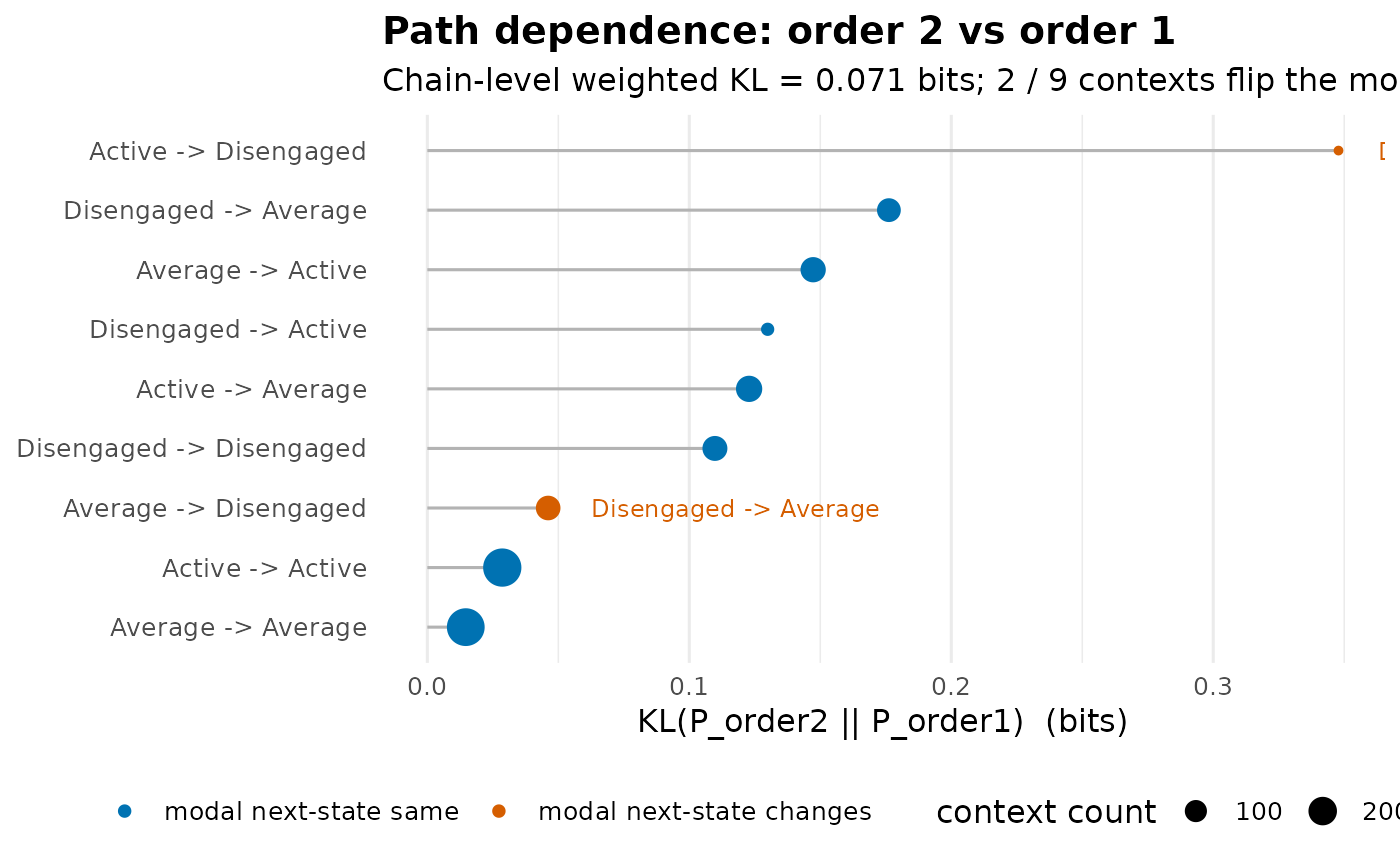
plot.net_path_dependence(): Lollipop chart of per-context KL divergence, sorted descending. Point size is proportional to context count; points where the modal next state flips between orders are marked with an X to highlight substantively meaningful order-2 effects.
References
Cover, T.M. & Thomas, J.A. (2006). Elements of Information Theory, 2nd ed., chapters 2 and 4. Wiley. (KL divergence and conditional entropy.)
Examples
data(trajectories, package = "Nestimate")
pd <- path_dependence(as.data.frame(trajectories), order = 2)
print(pd)
#> Path Dependence (order 2 vs order 1, bits)
#>
#> Contexts: 9 (min_count = 5).  Modal-prediction flips: 2.
#> Chain-level KL_weighted      = 0.071 bits
#> Chain-level H_drop_weighted  = 0.087 bits
#>
#> Top 9 contexts by KL:
#>                   context   n H_order1 H_orderk H_drop    KL     top_o1
#>      Active -> Disengaged  23    1.403    1.574 -0.171 0.348 Disengaged
#>     Disengaged -> Average 122    1.354    1.352  0.003 0.176    Average
#>         Average -> Active 144    1.040    1.125 -0.084 0.147     Active
#>      Disengaged -> Active  29    1.040    1.361 -0.321 0.130     Active
#>         Active -> Average 160    1.354    1.365 -0.011 0.123    Average
#>  Disengaged -> Disengaged 139    1.403    1.156  0.247 0.110 Disengaged
#>     Average -> Disengaged 134    1.403    1.430 -0.027 0.046 Disengaged
#>          Active -> Active 433    1.040    0.849  0.191 0.029     Active
#>        Average -> Average 419    1.354    1.229  0.126 0.015    Average
#>      top_ok flips
#>      Active  TRUE
#>     Average FALSE
#>      Active FALSE
#>      Active FALSE
#>     Average FALSE
#>  Disengaged FALSE
#>     Average  TRUE
#>      Active FALSE
#>     Average FALSE
summary(pd)
#> Path Dependence Summary (order 2 vs order 1, bits)
#>
#> All 9 contexts (sorted by KL):
#>                   context   n H_order1 H_orderk H_drop    KL     top_o1
#>      Active -> Disengaged  23    1.403    1.574 -0.171 0.348 Disengaged
#>     Disengaged -> Average 122    1.354    1.352  0.003 0.176    Average
#>         Average -> Active 144    1.040    1.125 -0.084 0.147     Active
#>      Disengaged -> Active  29    1.040    1.361 -0.321 0.130     Active
#>         Active -> Average 160    1.354    1.365 -0.011 0.123    Average
#>  Disengaged -> Disengaged 139    1.403    1.156  0.247 0.110 Disengaged
#>     Average -> Disengaged 134    1.403    1.430 -0.027 0.046 Disengaged
#>          Active -> Active 433    1.040    0.849  0.191 0.029     Active
#>        Average -> Average 419    1.354    1.229  0.126 0.015    Average
#>      top_ok flips
#>      Active  TRUE
#>     Average FALSE
#>      Active FALSE
#>      Active FALSE
#>     Average FALSE
#>  Disengaged FALSE
#>     Average  TRUE
#>      Active FALSE
#>     Average FALSE
#>
#> Chain-level:
#>  KL_weighted H_drop_weighted n_contexts n_flips
#>        0.071           0.087          9       2
plot(pd)