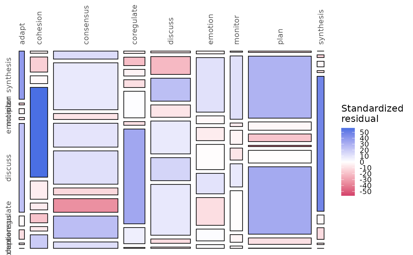
Mosaic Plot of a Network's Transition or Co-occurrence Counts
Source:R/plot_state_frequencies.R
mosaic_plot.RdDraws a Hartigan-Friendly mosaic (marimekko geometry, chi-square
standardized-residual fill) for an integer-weighted network. Equivalent in
algorithm and appearance to tna::plot_mosaic(); named differently to
avoid an export clash when both packages are attached.
Usage
mosaic_plot(x, ...)

# Default S3 method
mosaic_plot(x, ...)

# S3 method for class 'netobject'
mosaic_plot(
  x,
  xlab = NULL,
  ylab = NULL,
  range = NULL,
  top_angle = NULL,
  left_angle = NULL,
  residuals = c("permutation", "asymptotic"),
  n_perm = 500L,
  seed = NULL,
  values = FALSE,
  style = c("classic", "flat"),
  ...
)

# S3 method for class 'htna'
mosaic_plot(
  x,
  xlab = NULL,
  ylab = NULL,
  range = NULL,
  top_angle = NULL,
  left_angle = NULL,
  residuals = c("permutation", "asymptotic"),
  n_perm = 500L,
  seed = NULL,
  values = FALSE,
  style = c("classic", "flat"),
  ...
)

# S3 method for class 'mcml'
mosaic_plot(
  x,
  level = c("macro", "clusters"),
  xlab = NULL,
  ylab = NULL,
  range = NULL,
  top_angle = NULL,
  left_angle = NULL,
  residuals = c("permutation", "asymptotic"),
  n_perm = 500L,
  seed = NULL,
  ncol = 2L,
  values = FALSE,
  style = c("classic", "flat"),
  ...
)

# S3 method for class 'netobject_group'
mosaic_plot(
  x,
  xlab = NULL,
  ylab = NULL,
  range = NULL,
  top_angle = NULL,
  left_angle = NULL,
  residuals = c("permutation", "asymptotic"),
  n_perm = 500L,
  seed = NULL,
  ncol = 2L,
  values = FALSE,
  style = c("classic", "flat"),
  ...
)

# S3 method for class 'table'
mosaic_plot(
  x,
  xlab = "Row",
  ylab = "Column",
  range = NULL,
  top_angle = NULL,
  left_angle = NULL,
  residuals = c("permutation", "asymptotic"),
  n_perm = 500L,
  seed = NULL,
  values = FALSE,
  style = c("classic", "flat"),
  ...
)

# S3 method for class 'matrix'
mosaic_plot(x, ...)
Arguments
- x
One of the four data-bearing Nestimate classes:
netobject(single mosaic of$weights),netobject_group(one panel per group),mcml(between-cluster mosaic by default; per-cluster panels withlevel = "within"), orhtna(single mosaic of$weights; htna inherits netobject so the geometry matches). Also accepts a contingencytableor plain numericmatrixfor ad-hoc plotting.- ...
Flat styling overrides forwarded to the flat renderer when
style = "flat"(otherwise ignored).- xlab, ylab
Axis labels.
NULL(default) draws no axis title on the four data-bearing methods; thetable/matrixmethods default to"Row"and"Column". Pass any string to set one.- range
Numeric of length 2 giving the lower and upper colour-scale limits for the standardized residual.
NULL(default) auto-fits the limits to the symmetric rangec(-M, M)whereM = max(|stdres|)floored at 1, so no signal is squished and the legend stays readable on a near-independent table. Pass an explicit range (e.g.c(-4, 4)for tna-style display,c(-6, 6)for moderate clipping) to clamp the colour scale.- top_angle, left_angle
Rotation in degrees for the top (x) and left (y) tick labels.
NULL(default) uses the auto rule90 if n_levels > 3 else 0on each axis. Pass any numeric to override (e.g.top_angle = 45, left_angle = 0).- residuals
One of
"permutation"(default) or"asymptotic"."permutation"computes empirical-null z-scores by shuffling one variable's labels against the other forn_permdraws and reporting(O - mean_perm) / sd_permper cell. Robust on sparse tables."asymptotic"returnsstats::chisq.test()$stdres(the closed-form(O - E) / sqrt(E*(1 - p_row)*(1 - p_col))that vcd and tna use).- n_perm
Number of permutations when
residuals = "permutation". Default 500; use>= 1000for stable tail estimates.- seed
Optional integer seed for the permutation RNG. Use for reproducible plots; ignored when
residuals = "asymptotic".- values
Logical. When
TRUE, overlay each cell's standardized residual as a numeric label (one decimal). Text colour switches to white on saturated cells (|stdres| > 1.5) and dark grey otherwise. DefaultFALSE– the colour bar legend already conveys the sign and magnitude.- style
Character.
"classic"(default) draws the black-borderedtheme_minimalmosaic with axis labels;"flat"draws the flattheme_voidmosaic with white gutters, a soft background and a colour-bar legend. Withstyle = "flat",values = TRUEprints the standardized residual inside each tile, and extra flat styling arguments (tile_label,col_label_side,row_label_side,legend_position,legend_size,label_size, ...; seemosaic_analysis) may be passed via.... Not supported for multi-panelmcml(level = "clusters"), which falls back to the classic faceted style.- level
For
mcmlonly."macro"(default) draws a single mosaic ofx$macro$weights(the cluster-by-cluster aggregate);"clusters"draws one mosaic per cluster fromx$clusters[[k]]$weights, faceted into one combined ggplot.- ncol
Number of columns in the multi-panel layout. Default 2. Effective only for
mcmlwithlevel = "clusters", the one multi-panel case;netobject_groupis drawn as a single (group x state) mosaic, soncolis accepted but has no effect there.
Value
A ggplot object: one geom_rect layer with one
rectangle per contingency-table cell, filled by the standardized
residual. mcml with level = "clusters" returns a single
facet_wrap-ed ggplot (one panel per cluster, shared fill
scale); every other input returns a single-panel ggplot.
Details
Column widths are proportional to row marginals of the weight matrix
(incoming totals when the matrix is transposed, as for transitions). Within
each column, segment heights are proportional to that row's conditional
distribution. Cell fill is the standardized residual under the independence
null – a permutation z-score by default, or the closed-form
stats::chisq.test() residual with residuals = "asymptotic"
(see residuals) – on a diverging palette whose limits auto-fit the
observed residuals unless range is supplied.
Mosaics need integer counts: when $weights is already integer
(method = "frequency" / "co_occurrence") it is used directly;
for a single netobject / htna otherwise (relative, glasso,
cor, ...) order-1 transition counts are recounted from the raw $data
sequences. The function errors only when neither integer weights nor
$data are available.
See also
plot_mosaic for the lower-level data.frame primitive.
Examples
data(group_regulation_long, package = "Nestimate")
net <- build_network(group_regulation_long, method = "frequency",
                     format = "long", actor = "Actor", action = "Action",
                     order = "Time")
mosaic_plot(net, seed = 1)