tsn

tsn constructs networks from time-series data. Representing a time series as a network exposes its temporal structure to the tools of graph theory, and several established methods do this in different ways. What distinguishes them is what each node represents; tsn collects them under a single interface and a single result object.

Whatever the input, a single time series or a collection of them, the analysis follows one of two paths that differ only in what becomes a node:

                        ┌─►  states ───────────────────────►  transition network
  a univariate series ──┤
  (one or several)      └─►  series, windows, or points  ──►  distance or
                             (individual observations)        visibility network

Two broad strategies are supported:

• Nodes are states. A numeric series is discretized into a small alphabet of states, and the network encodes how the series moves between those states over time. The result is a state-transition network.
• Nodes are the measurements themselves, whether a whole series, a sliding window, or an individual observation. Edges are then defined directly by the distance or the visibility relation between nodes, with no discretization step.

The exported functions cover both strategies:

Task	Function(s)	Options
Model state transitions	ts_tna(), ts_ftna(), ts_cna(), ts_atna()	transition probabilities, frequencies, co-occurrences, or attention-weighted transitions (via Nestimate)
Split a pooled model by series	series_networks()	one network per series
Discretize values into states	discretize() (or tsn(unit = "state"))	15 discretizers, applied consistently across series
Classify local trend direction	trend()	Theil–Sen (default), OLS, Spearman, or Kendall slope; growth factor
Build a distance or visibility network	tsn(), vg()	15 distance measures; natural or horizontal visibility; full, nearest-neighbour, threshold, percentile, or Gaussian connectivity

Related packages. tsn is distinct from tsnet (Bayesian graphical vector autoregression), tsna (temporal social-network analysis), and ts2net (a related time-series-to-network toolkit). Its emphasis is a compact, dependency-light interface that supports irregularly spaced visibility graphs, fifteen discretizers, and an optional bridge to transition-network models.

Installation

The package is not currently published on CRAN. Install the development release from GitHub:

install.packages("remotes")
remotes::install_github("mohsaqr/tsn")

State-transition networks

The ts_tna() family constructs a transition network directly from raw measurements: each series is discretized, a single state alphabet is shared across all series, and the estimation is delegated to Nestimate (a Suggests dependency). The four functions differ only in the quantity placed on the edges. ts_tna() estimates transition probabilities, ts_ftna() raw transition frequencies, ts_cna() co-occurrences, and ts_atna() attention-weighted transitions.

The packaged steps dataset records daily step counts. Because participant 35 has missing days, we model the complete observations for two participants:

data(steps)

complete <- subset(steps, !is.na(steps))

model <- ts_tna(
  complete,
  value = "steps",
  id = "id",
  time = "day",
  series = c(536, 88),
  n_states = 3,
  labels = c("low", "moderate", "high")
)

model
#> Transition Network (relative probabilities) [directed]
#>   Weights: [0.108, 0.605]  |  mean: 0.333
#> 
#>   Weight matrix:
#>              low moderate  high
#>   low      0.578    0.303 0.119
#>   moderate 0.319    0.411 0.270
#>   high     0.108    0.286 0.605 
#> 
#>   Initial probabilities:
#>   high          1.000  ████████████████████████████████████████
#>   low           0.000  
#>   moderate      0.000

The transition matrix is strongly diagonal: in the pooled model a low day is followed by another low day with probability 0.578, and a high day by another high day with probability 0.605, so days tend to persist in their state. Because the state alphabet is learned from both series jointly, the two participants are placed on a common scale. series_networks() then splits the pooled model into one network per series:

series_networks(model)
#>  series type observations states edges
#>      88  tna          292      3     9
#>     536  tna          265      3     9

The resulting collection supports print(), summary(), as.data.frame(), and plot() directly (plot() takes series = "<name>" when the collection holds more than one model). The combined plot places each participant’s shaded series alongside their own transition network:

plot(model, ribbon = TRUE, overlay = "none")
#> Registered S3 method overwritten by 'cograph':
#>   method     from     
#>   print.mcml Nestimate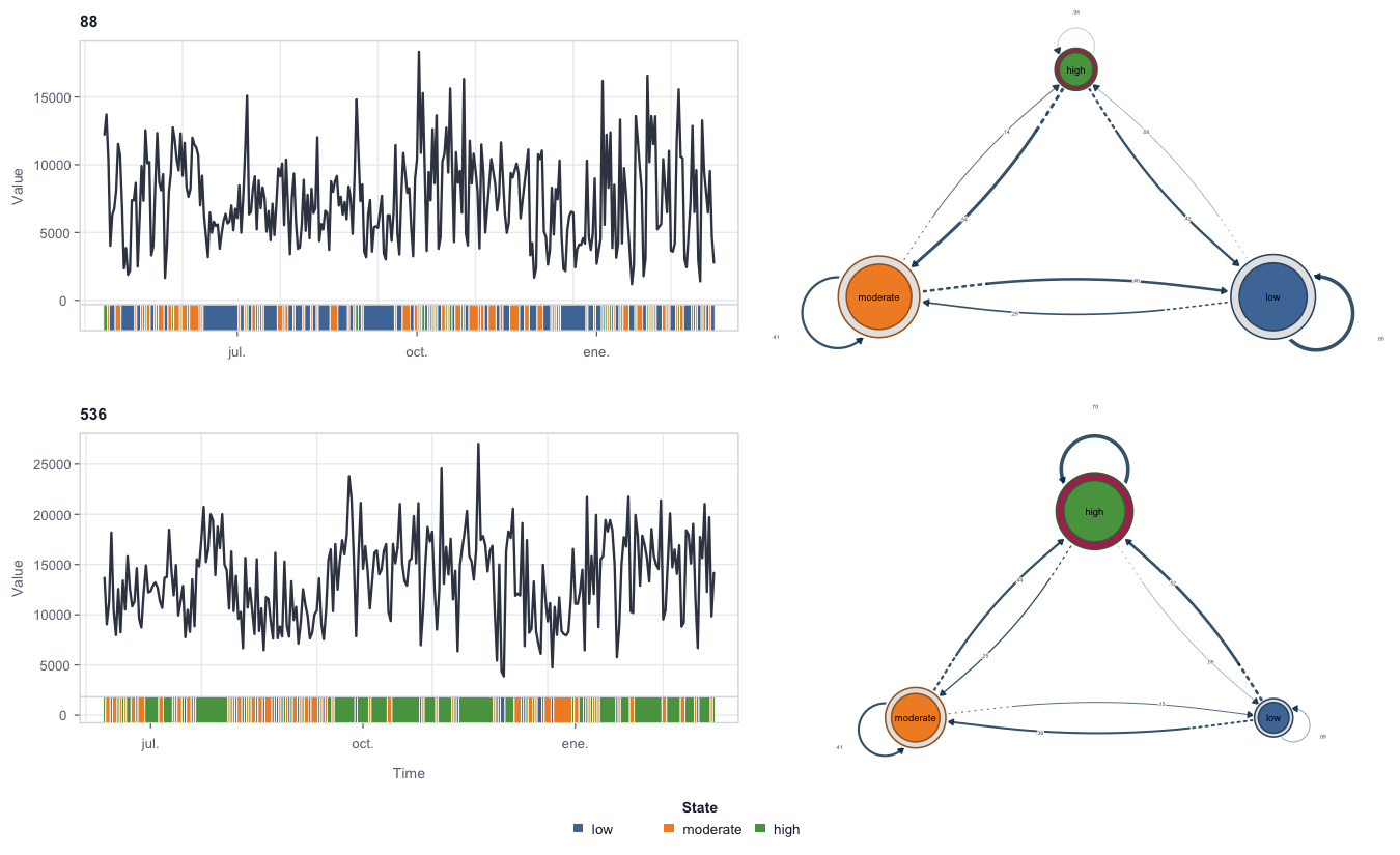

Because the result is a genuine Nestimate model, the full range of downstream Nestimate tools applies unchanged (for example Nestimate::net_centrality(model)). Inferential procedures retain their usual sampling requirements; sequence bootstrap, in particular, is not informative for a model estimated from a single sequence.

From values to states: discretize() and trend()

discretize() is the bridge from a numeric series to a state sequence. Using the same steps data, participant 536 contributes 265 complete days:

states <- discretize(
  steps,
  value = "steps",
  id = "id",
  time = "day",
  series = 536,
  method = "quantile",
  n_states = 3,
  labels = c("low", "moderate", "high")
)

summary(states)
#>      state count proportion mean_value
#> 1      low    88  0.3320755   8838.966
#> 2 moderate    89  0.3358491  13599.753
#> 3     high    88  0.3320755  18165.034

Fifteen discretizers are available (threshold, width, quantile, kde, kmeans, gaussian, hclust, ordinal, symbolic, change_points, entropy, magnitude, adaptive_magnitude, percentile_magnitude, dtw). The temporal discretizers are group-aware: ordinal patterns, adaptive-magnitude features, and DTW windows are computed separately within each series and then mapped onto one shared state vocabulary, so that states remain comparable across series.

trend() is a companion discretizer for direction rather than level: it classifies each observation by the slope of a rolling regression.

movement <- trend(
  steps,
  value = "steps",
  id = "id",
  time = "day",
  series = 536,
  window = 14
)

summary(movement)
#>        state count proportion
#> 1  Ascending    91  0.3433962
#> 2 Descending    80  0.3018868
#> 3  Turbulent    81  0.3056604
#> 4    Initial    13  0.0490566

Visibility networks: observations as nodes

A visibility graph (Lacasa et al., 2008) maps a single series onto a network of its observations: two time points are connected when an unobstructed straight sightline over the intervening values joins them. The packaged motivation dataset holds 4,871 experience-sampling measurements; the first 60 pleasure ratings suffice to illustrate the construction.

data(motivation)

pleasure <- head(motivation, 60)
network <- vg(pleasure, series = "pleasure")

summary(network)
#>       method unit nodes dyads edges    density minimum_weight maximum_weight
#> 1 visibility time    60   143   143 0.08079096              1              1
#>   directed
#> 1    FALSE

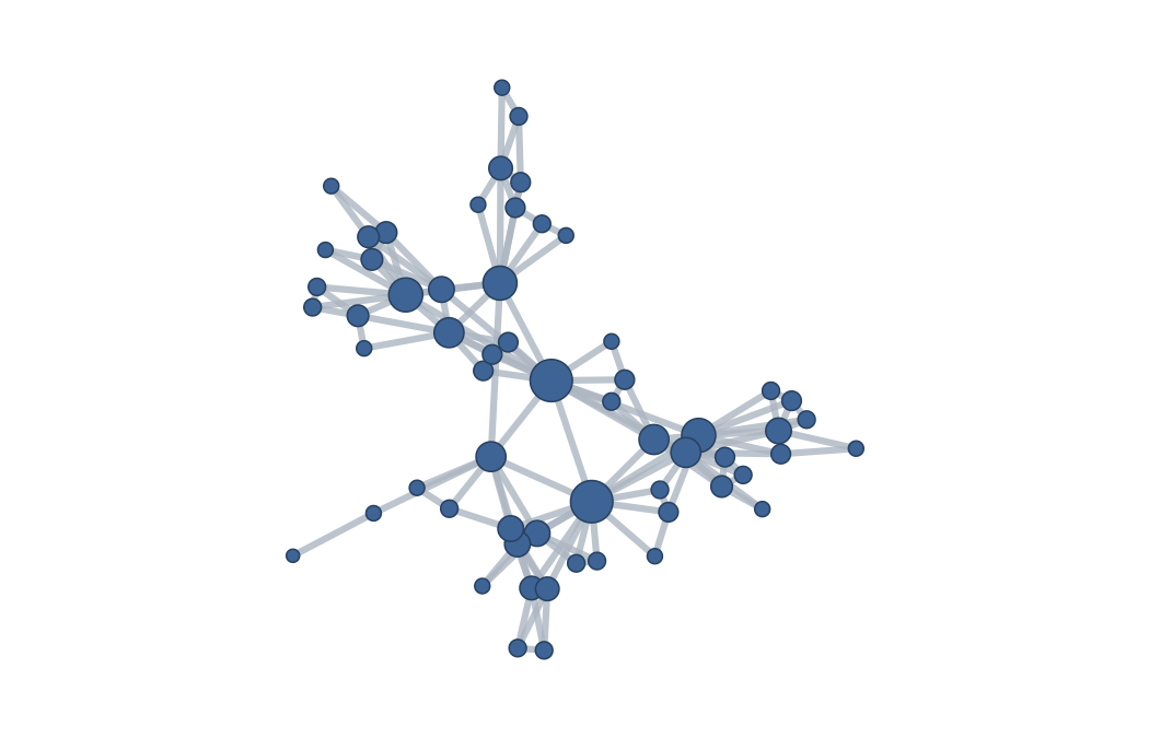
The 60 observations become 60 nodes joined by 143 sightlines. Every network offers two complementary views: plot(x) draws the network itself through cograph, and plot(x, "series") shows the source series from which it was built.

plot(network, layout = "fr", node_size_range = c(1.4, 4.5))

plot(network, "series")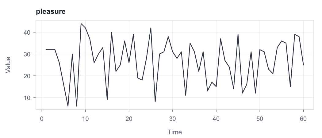

vg(x) builds a natural visibility graph and vg(x, "horizontal") a horizontal one (Luque et al., 2009); the tsn() shortcuts "nvg" and "hvg" are equivalent. Visibility options include directed, penetrable (sightlines may cross a bounded number of points), limit (a maximum elapsed time), and decay. When a time column is supplied, both the sightlines and the elapsed-time rules respect the observed spacing between points, which may be irregular, rather than mere row positions.

State networks from visibility

tsn(unit = "state") applies the same discretization engine and then projects the visibility graph onto the states: nodes become states, and each edge aggregates (by default, sums) the sightlines between occurrences of a state pair.

state_network <- tsn(
  steps,
  value = "steps",
  id = "id",
  time = "day",
  series = 536,
  unit = "state",
  discretization = "quantile",
  n_states = 3
)

summary(state_network)
#>       method  unit nodes dyads edges density minimum_weight maximum_weight
#> 1 visibility state     3     6     6       1             56            258
#>   directed
#> 1    FALSE

The series view shades the states over the raw values, either as horizontal value bands (overlay = "horizontal") or as vertical runs along time:

plot(state_network, "series", overlay = "horizontal")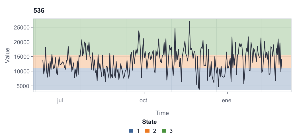

Distance networks: series and windows as nodes

Under method = "distance", nodes are whole series (or sliding windows) and edge weights are similarities, so that larger weights indicate closer series. Comparing five motivation variables as complete series is a single call:

affect <- tsn(
  motivation,
  series = c("pleasure", "autonomy", "competence", "relatedness", "mood"),
  method = "distance",
  distance = "correlation"
)

summary(affect)
#>     method   unit nodes dyads edges density minimum_weight maximum_weight
#> 1 distance series     5    10    10       1      0.5088532      0.6586452
#>   directed
#> 1    FALSE

plot(affect, labels = TRUE)

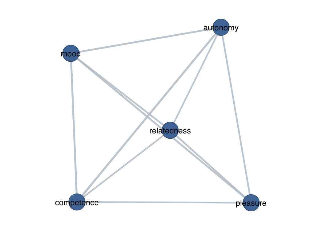
All ten pairs are connected because the default connectivity rule is connect = "full"; autonomy and competence form the closest pair. Fifteen distance measures are available (euclidean, manhattan, maximum, canberra, minkowski, binary, cosine, correlation, spearman, dtw, ccf, nmi, voi, event_sync, van_rossum), and connect sparsifies the network by nearest neighbours, a distance threshold, a percentile, or a Gaussian kernel.

The same function compares sliding windows of a single series, turning one trajectory into a network of its own epochs:

windows <- tsn(
  pleasure,
  series = "pleasure",
  method = "distance",
  distance = "dtw",
  window = 12,
  step = 4,
  connect = "nearest",
  neighbors = 2
)

summary(windows)
#>     method   unit nodes dyads edges   density minimum_weight maximum_weight
#> 1 distance window    13    78    17 0.2179487     0.00990099     0.02564103
#>   directed
#> 1    FALSE

The 60 ratings yield 13 overlapping windows; retaining each window’s two nearest neighbours keeps 17 of the 78 possible dyads. The default window is 10% of the series length, so step should be chosen relative to the series length. Further options include chain = TRUE (connect only consecutive windows or series), directed = TRUE, and normalize = TRUE.

A single object, a consistent grammar

However it was constructed, a tsn network is the same kind of object: a list-backed result carrying the netobject and cograph_network classes, with a tidy dyad table inside. The standard methods apply throughout:

summary(network)                         # one tidy row describing the network
as.data.frame(network)                   # the dyad table
as.data.frame(network, what = "series")  # the source observations
as.matrix(network)                       # the weighted adjacency matrix

plot(network)                            # network view, rendered by cograph
plot(network, "series")                  # source-series view, base graphics

plot() on a network applies readable defaults (a spring layout with degree-scaled nodes); any cograph argument passes straight through and overrides them, for example plot(network, layout = "circle", labels = TRUE).

Vignettes

• vignette("nestimate-workflow") builds a transition-network model from a series and tests it with Nestimate: bootstrap confidence intervals, centrality stability, a Markov-order test, and a permutation test comparing two periods.
• vignette("pleasure-all-functions") applies every exported tsn function to the packaged motivation pleasure series, building each network representation in turn.
• vignette("plotting-time-series-networks") documents the plotting surface: the network and source-series views, state overlays, and transition-model plots.

Relationships with other packages

tsn focuses on turning time series into networks and relies on base R alone for that core. Two related tasks are handled by companion packages:

• Nestimate (Saqr, López-Pernas, & Misiejuk, 2026) estimates and analyses transition networks, following the transition-network-analysis framework of Saqr et al. (2025). The ts_tna() family discretizes the raw series and then calls its builders, so a tsn transition network is itself a Nestimate model that every Nestimate method applies to.
• cograph (Saqr, López-Pernas, & Tikka, 2026) provides graph conversion, analytics, layout, and rendering. Because every tsn result already carries the cograph_network class, plot(network) delegates to cograph::splot().

Both are Suggests: Nestimate is needed only for transition networks and cograph (with igraph) only for network plots. Everything else runs on a base-R installation.

References

Lacasa, L., Luque, B., Ballesteros, F., Luque, J., & Nuño, J. C. (2008). From time series to complex networks: The visibility graph. Proceedings of the National Academy of Sciences, 105(13), 4972–4975. https://doi.org/10.1073/pnas.0709247105

Luque, B., Lacasa, L., Ballesteros, F., & Luque, J. (2009). Horizontal visibility graphs: Exact results for random time series. Physical Review E, 80, 046103. https://doi.org/10.1103/PhysRevE.80.046103

Saqr, M., López-Pernas, S., Törmänen, T., Kaliisa, R., Misiejuk, K., & Tikka, S. (2025). Transition network analysis: A novel framework for modeling, visualizing, and identifying the temporal patterns of learners and learning. Proceedings of the 15th Learning Analytics and Knowledge Conference. https://doi.org/10.1145/3706468.3706513

Saqr, M., López-Pernas, S., & Misiejuk, K. (2026). Nestimate: Network estimation, bootstrap, and higher-order analysis. R package version 0.8.4. https://github.com/mohsaqr/nestimate

Saqr, M., López-Pernas, S., & Tikka, S. (2026). cograph: Analysis and visualization of complex networks. R package version 2.4.5. https://github.com/sonsoleslp/cograph

Authors

• Mohammed Saqr, University of Eastern Finland · saqr.me
• Sonsoles López-Pernas, University of Eastern Finland · sonsoles.me
• Manuel J. Gómez, University of Murcia · manueljgomez.es

License

MIT