Plot latents results

plot() draws any result of this package and returns a ggplot object, which can be printed, saved with ggplot2::ggsave() or restyled with + ggplot2::theme(). The plots of mixture regressions (for fits that classify persons, the "fitted" view only), pooled imputations and bootstrap tests are drawn when called, including inside loops, and their ggplot is returned invisibly.

Usage

# S3 method for class 'latents_family_enumeration'
plot(
  x,
  what = c("bic", "aic", "bic_individual"),
  main = NULL,
  subtitle = NULL,
  criterion = NULL,
  ...
)

# S3 method for class 'multilpa_additive'
plot(
  x,
  what = c("means", "variances", "intercepts"),
  level = 0.95,
  main = NULL,
  subtitle = NULL,
  ...
)

# S3 method for class 'latents_comparison'
plot(x, main = NULL, subtitle = NULL, ...)

# S3 method for class 'multilpa_cross_level'
plot(
  x,
  what = c("profiles", "group_means", "composition"),
  main = NULL,
  subtitle = NULL,
  ...
)

# S3 method for class 'multilpa_bootstrap_lrt'
plot(x, main = NULL, subtitle = NULL, palette = NULL, style = NULL, ...)

# S3 method for class 'latents_growth_mixture'
plot(
  x,
  what = c("trajectories", "individuals", "coefficients", "random", "classification",
    "posteriors"),
  time = NULL,
  facet = FALSE,
  persons = 12L,
  max_persons = 120L,
  spread = 0.8,
  level = 0.95,
  main = NULL,
  subtitle = NULL,
  ...
)

# S3 method for class 'latents_transition_enumeration'
plot(
  x,
  what = c("bic", "aic", "bic_individual"),
  main = NULL,
  subtitle = NULL,
  criterion = NULL,
  ...
)

# S3 method for class 'multilpa_lta'
plot(x, main = NULL, subtitle = NULL, ...)

# S3 method for class 'latents_regression_enumeration'
plot(
  x,
  what = c("aic", "bic", "sabic", "icl"),
  combine = TRUE,
  labels = TRUE,
  mark_minimum = TRUE,
  main = NULL,
  subtitle = NULL,
  cutoff = 0.8,
  using = "bic",
  ...
)

# S3 method for class 'latents_mixture_regression'
plot(
  x,
  what = NULL,
  predictor = NULL,
  level = 0.95,
  main = NULL,
  subtitle = NULL,
  time = NULL,
  facet = FALSE,
  persons = 12L,
  max_persons = 120L,
  ...
)

plot_profiles(
  x,
  statistic = c("mean", "median", "mode"),
  scale = c("raw", "standardized"),
  intervals = TRUE,
  labels = TRUE,
  data = NULL,
  main = NULL,
  subtitle = NULL,
  what = c("lines", "bars", "heatmap", "raincloud", "parallel", "pairs", "all")
)

plot_responses(
  x,
  category = "last",
  intervals = TRUE,
  labels = TRUE,
  data = NULL,
  main = NULL,
  subtitle = NULL
)

plot_sequences(
  x,
  labels = TRUE,
  cell_labels = TRUE,
  main = NULL,
  subtitle = NULL
)

plot_prevalence(x, labels = TRUE, main = NULL, subtitle = NULL)

plot_diagnostics(
  x,
  what = c("all", "sizes", "posteriors", "entropy", "avepp", "group_sizes",
    "group_posteriors", "group_entropy", "group_avepp"),
  main = NULL,
  subtitle = NULL
)

plot_transitions(x, main = NULL, subtitle = NULL)

plot_tree(
  x,
  main = NULL,
  subtitle = NULL,
  n_group_classes = NULL,
  n_profiles = NULL,
  model = NULL,
  candidates = NULL,
  from = NULL,
  to = NULL,
  level = c("individuals", "groups"),
  combine = FALSE
)

plot_selection(
  x,
  what = c("all", "deltas", "heatmap", "smallest", "trust", "diagnostics"),
  using = "bic_groups",
  cutoff = 0.8,
  main = NULL,
  subtitle = NULL
)

# S3 method for class 'multilpa'
plot(
  x,
  what = c("profiles", "bars", "heatmap", "raincloud", "parallel", "pairs", "responses",
    "probabilities", "sequences", "sizes", "entropy", "posteriors", "avepp", "all"),
  data = NULL,
  scale = c("raw", "standardized"),
  category = "last",
  labels = TRUE,
  intervals = TRUE,
  cell_labels = TRUE,
  main = NULL,
  subtitle = NULL,
  statistic = c("mean", "median", "mode"),
  ...
)

# S3 method for class 'multilpa_enumeration'
plot(
  x,
  what = c("aic", "bic_groups", "bic_individual", "icl_individual"),
  criterion = NULL,
  combine = TRUE,
  labels = TRUE,
  mark_minimum = TRUE,
  main = NULL,
  subtitle = NULL,
  cutoff = 0.8,
  using = "bic_groups",
  ...
)

plot_enumeration(
  x,
  what = c("aic", "bic_groups", "bic_individual", "icl_individual"),
  combine = TRUE,
  labels = TRUE,
  mark_minimum = TRUE,
  main = NULL,
  subtitle = NULL,
  cutoff = 0.8,
  using = "bic_groups",
  ...
)

# S3 method for class 'multilpa_covariates'
plot(
  x,
  what = c("profiles", "bars", "heatmap", "raincloud", "parallel", "pairs", "responses",
    "sequences", "sizes", "entropy", "posteriors", "avepp", "all"),
  data = NULL,
  scale = c("raw", "standardized"),
  category = "last",
  labels = TRUE,
  intervals = TRUE,
  cell_labels = TRUE,
  main = NULL,
  subtitle = NULL,
  statistic = c("mean", "median", "mode"),
  ...
)

plot_views(x = NULL)

# S3 method for class 'latents_pooled'
plot(
  x,
  what = c("profile", "group", "measurement"),
  main = NULL,
  subtitle = NULL,
  level = NULL,
  ...
)

# S3 method for class 'multilpa_transitions'
plot(
  x,
  what = c("transitions", "profiles", "bars", "heatmap", "responses", "sequences",
    "sizes", "entropy", "posteriors", "avepp", "all"),
  data = NULL,
  scale = c("raw", "standardized"),
  category = "last",
  labels = TRUE,
  cell_labels = TRUE,
  main = NULL,
  subtitle = NULL,
  intervals = TRUE,
  ...
)

Arguments

x

The object to plot. For plot_profiles(), plot_responses(), plot_sequences(), plot_prevalence(), plot_diagnostics() and plot_transitions(), any fitted model of the package: profile, class and transition models from multilpa(), multilca(), lpa(), lca() and lta() (with or without covariates) take the views described under what and What plot() draws; growth mixtures and mixture regressions from mixture_regression(), additive, dispersion and cross-level fits from multilpa(), pooled imputations from pool_imputations() and general lta() fits (occasion-varying transitions, covariates, mover-stayer, second order, weights, ordinal or count indicators) take the views listed under Named plot functions on other fitted models. For plot_enumeration(), plot_selection() and plot_tree(), a grid from enumerate_classes(), enumerate_lpa(), enumerate_lca() or enumerate_regressions(); each refuses the views that grid does not offer (see above). Optionally a grid for plot_views().

what

The view to draw. "all" draws every view of that function that the model supports, as a list, and names in a message any it cannot draw. On fitted models other than profile, class and transition models, plot_profiles() draws only "lines" and plot_diagnostics() only "posteriors", where that model has the view (see Named plot functions on other fitted models). For plot_profiles(): "lines" (default), "bars" (means from zero with 95% intervals), "heatmap" (means in observed standard deviations, or the response probabilities of categorical indicators), "raincloud" (each indicator's distribution by assigned profile), "parallel" (every case as a line) or "pairs" (scatter-plot matrix with each profile's 95% covariance ellipse).

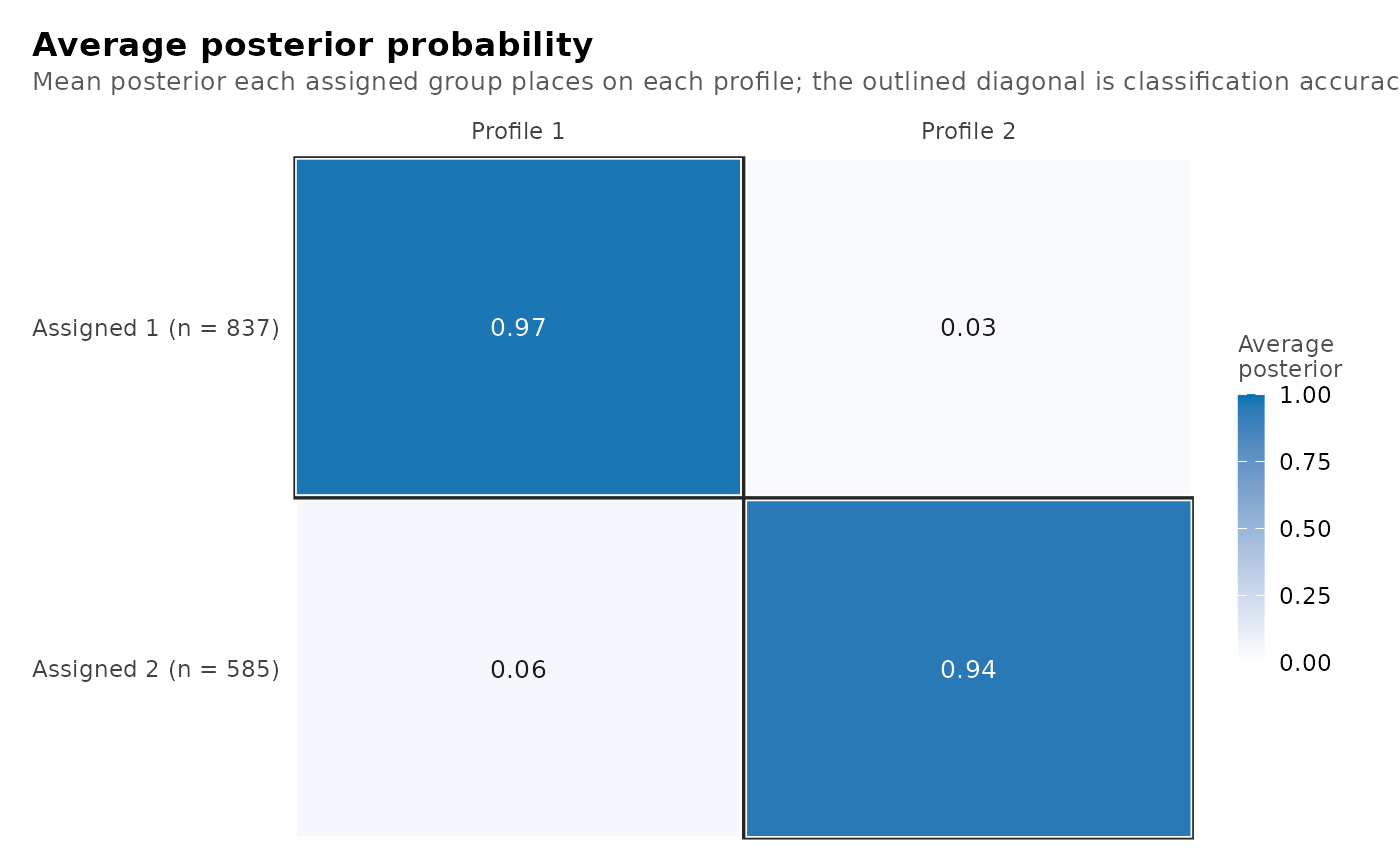
For plot_diagnostics(): "all" (default), "sizes" (effective profile counts), "posteriors" (posterior probability of each case's assigned profile), "entropy" (each case's entropy relative to a flat posterior) or "avepp" (average posterior probability matrix). "group_sizes", "group_posteriors", "group_entropy" and "group_avepp" draw the same four views for the groups and their group classes; "all" includes them when the fit has two or more group classes, and with fewer they are refused with latents_no_group_classes. A fit with a noise component supports "sizes" and the group views only: "all" returns "sizes", and the other individual-level views are refused with latents_unsupported_noise.

For plot_selection(): "all" (default), "deltas", "heatmap", "smallest", "trust" or "diagnostics", as described for plot_enumeration().

For plot_enumeration(), three kinds of view; information criteria cannot be requested together with the other two:

Information criteria: criterion columns of as.data.frame(x), such as "bic_groups", or "all". On a profile or class grid the default draws AIC, both BICs and ICL over individuals; on a transition or family grid AIC, BIC and BIC over individuals; on a regression grid AIC, BIC, SABIC and ICL.
Classification quality across the candidates, at each level with two or more classes: "entropy" (relative entropy), "avepp" (the lowest AvePP, with the cutoff dashed) or "diagnostics" (both).
Model-selection evidence (none of which selects a model): "deltas" (the decrease in the criterion in using with each added profile and each added group class; see get_results(x, "deltas") and "knees"), "heatmap" (the criterion over profiles and group classes, relative to the lowest), "smallest" (the smallest class share, with 5% dashed) or "trust" (convergence, boundary and replication of every candidate). "selection" draws all four and "diagnostics", as a list.

main, subtitle

Title and subtitle. NULL (default) uses the view's own.

criterion

The former name of what for enumeration criteria. On a profile grid it is used alone or with what = "enumeration"; transition and group-class family grids take "bic", "aic" or "bic_individual" (or a unique abbreviation, such as "bic_i"), or any other view of the grid.

...

With what = "tree" (on plot() of an enumeration or on plot_enumeration()), the arguments of plot_tree(). On plot() of a transition or group-class family grid, also combine, labels, mark_minimum, cutoff and using, passed to plot_enumeration(). Otherwise not used. Profile, class and transition models and enumerations refuse unknown arguments with latents_bad_argument; the other methods ignore them with a latents_unused_argument warning (see Errors).

level

For plot_tree(), "individuals" (default; the cases divided into profiles or classes) or "groups" (the groups divided into group classes). Otherwise the confidence level for additive, mixture-regression and growth views (default 0.95). On pooled plots, the former name of what: "profile", "group" or "measurement".

palette

For bootstrap plots, a colour vector for the histogram and the observed statistic; NULL (default) uses the standard colours.

style

The former bootstrap drawing style; ignored with a latents_unused_argument warning.

time

For growth and trajectory views, the numeric time column. NULL (default) uses the first numeric variable in the fitted random or regression design.

facet

For trajectories, FALSE (default) draws all classes in one panel; TRUE draws one panel per class.

persons

For individual trajectories, the number of persons to show (default 12), or a vector of their identifiers.

max_persons

The maximum number of observed trajectories drawn behind the class means (default 120); zero hides them.

spread

For growth trajectories, the band of random-effect spread of persons around the class curve, from 0 (hidden) to less than 1; default 0.8.

combine

TRUE (default) draws several criteria as panels of one plot; FALSE returns one plot per criterion. For plot_tree() (and what = "tree"), FALSE (default) returns one plot per tree and TRUE draws every tree as a panel of one plot.

labels

TRUE (default) labels each series directly; FALSE uses a legend. On sequence views, TRUE groups the rows by group class under labelled strips.

mark_minimum

TRUE (default) circles each criterion's lowest value among converged candidates, without selecting a model. Information criteria only.

cutoff

For plot_enumeration(what = "avepp"), "diagnostics" or "selection", the AvePP cutoff drawn as a dashed line (default 0.8).

using

For plot_enumeration(what = "deltas"), "heatmap" or "selection", the information criterion used. When not given, a profile or class grid uses "bic_groups" and the other grids "bic"; "smallest" and "trust" use none.

predictor

For the fitted view of a mixture regression, a numeric predictor in the formula. NULL (default) uses the first numeric predictor.

statistic

"mean" (default), "median" or "mode". They coincide for continuous indicators; for categorical ones they summarise the fitted probabilities on the numeric category scale, without intervals.

scale

"raw" (default) keeps each indicator in its own units; "standardized" divides its deviation from the observed mean by its observed standard deviation.

intervals

For profile, bar and response views, TRUE (default) draws 95% intervals when the fit has standard errors; otherwise the subtitle states why there are none. They are the conf_low and conf_high of parameter_inference(); a response probability's interval is formed on the logit scale.

data

The data the model was fitted to, used only to compute the intervals. NULL (default) uses the data stored in the fit.

category

Which category's probability to draw: "last" (default), "first", or a single label or index.

cell_labels

For sequence views, TRUE (default) prints each assigned profile in its cell when the cells are large enough for the text.

n_group_classes, n_profiles, model

For plot_tree(), the trees and rows to draw. At the individual level a tree runs down the numbers of profiles (classes) at one number of group classes and one structure: n_group_classes and model choose trees, n_profiles the rows. At the group level a tree runs down the numbers of group classes at one number of profiles: n_profiles and model choose trees, n_group_classes the rows. NULL (default) keeps every converged candidate. A single count for the rows (n_profiles at the individual level, n_group_classes at the group level) is one level of every tree, and the plot compares that level's solutions instead: plot_tree(x, n_profiles = 4, n_group_classes = c(2, 5)) draws the four-profile solution at two and at five group classes as two rows, each class in the colour of the class it matches in the first row.

candidates

For plot_tree(), two or more candidate names drawn as the rows of one tree, in the order given, to compare those solutions. Not combined with n_group_classes, n_profiles or model.

from, to

For plot_tree(), two solutions to compare as a two-row tree, each named by its class counts c(n_profiles, n_group_classes) (one count means one group class) or by its name: plot_tree(x, from = c(3, 3), to = c(4, 3)). Given together, and not with candidates. On a grid crossed with covariance structures, model names the structure of both.

Value

A ggplot object. what = "all" (on plot() of a fitted model or on a named plot function), plot_enumeration(combine = FALSE) with several criteria or classification-quality measures, and enumeration views when more than one is requested (including "selection") return a latents_plots list of ggplot objects, which draws each one when printed, pausing between plots on an interactive screen device. plot_tree() and what = "tree" return one ggplot for a single tree or combine = TRUE, and otherwise a latents_plots list named by tree. plot_views() returns a data.frame with one row per view: type (the value for what), group and description. plot_views(x) of a grid returns one row per what value of that grid: type, group ("criteria", "quality", "selection" or "tree"), supported (TRUE when the grid offers it), description and reason (why it is not offered; NA when it is).

Details

The main views also have their own functions, each grouping related views under what, with "all" drawing every one: plot_profiles() (profile means as lines, bars, a heatmap, rainclouds, parallel lines or pairs, or categorical means, medians and modes), plot_responses() (categorical response probabilities), plot_sequences() (each group's profile at each occasion), plot_prevalence() (profile shares within each group class), plot_diagnostics() (classification quality), plot_transitions() (transition matrix), plot_enumeration() (information criteria, classification quality and model-selection evidence across a grid), plot_selection() (the model-selection evidence of a grid) and plot_tree() (how profiles split as more are added, one plot per tree, or how chosen solutions correspond). Each draws the same plot as the matching plot(x, what = ). The fit functions take every fitted model of the package; for growth mixtures, mixture regressions, additive and dispersion fits, cross-level fits, pooled imputations and general lta() fits they draw the view of that fit's own plot() that shows the same quantity, and refuse the rest (see Named plot functions on other fitted models). plot_views() lists the views of a fitted model, and "enumeration" and "tree" for a grid, with a one-line description of each; plot_views(grid) lists every view of that grid, whether it is offered, and why not.

The grid functions take every grid of the package: profile and class grids (enumerate_classes(), enumerate_lpa(), enumerate_lca()), transition grids (enumerate_classes(time = )), group-class family grids (enumerate_classes(family = )) and regression grids (enumerate_regressions()). Each kind offers the views its candidates carry:

View	Profiles, classes	Transitions	Families	Regressions
criteria	14 columns	aic, bic, bic_individual	aic, bic, bic_individual	aic, bic, bic_rows, sabic, icl
entropy, avepp, diagnostics	yes	yes	group classes	yes
deltas, heatmap, smallest, trust, selection	yes	yes	no	yes
tree	yes	yes	no	no

A family grid's candidates have group classes and no profiles, so its criteria and quality are drawn against the number of group classes, and the views laid out by profiles and group classes, and the tree, are not drawn. A regression grid's candidates are not named, so it has no tree; its smallest-class view reads the smallest_share of its table, and its trust view has no boundary column to read. A view a grid does not offer is refused with latents_unsupported_view.

Each profile keeps the same order (largest first), Okabe-Ito colour and point shape in every view. The plots require ggplot2, which is a suggested package.

What `plot()` draws

Each object takes what = for its views, main, subtitle and the arguments named here.

Fitted profile and class models: From multilpa(), multilca(), lpa(), lca() and covariate models: "profiles" (default), "bars", "heatmap", "raincloud", "parallel", "pairs" (each profile's 95% covariance ellipse), "responses", "probabilities" (not for covariate models), "sequences" (fits with time; cell_labels = TRUE prints the profile in each cell), "sizes", "entropy", "posteriors", "avepp" and "all". The profile views name in a caption any ordinal, count or (for the means) categorical indicator they omit.
Transition fits: From lta(): "transitions" (default), then "profiles", "bars", "heatmap", "responses", "sequences", "sizes", "entropy", "posteriors", "avepp" and "all", without statistic; the profile, bar and response views draw the 95% intervals of the transition fit's parameter_inference() (intervals). A general lta() fit takes no what and draws its transition matrix, which plot_transitions() draws too.
Enumerations: Criterion columns or "all" (with combine, labels and mark_minimum), "tree" (with the arguments of plot_tree()), the classification-quality views "entropy", "avepp" and "diagnostics" (with cutoff), and the model-selection views "deltas" and "heatmap" (which use the criterion in using), "smallest" and "trust"; "selection" draws those four and "diagnostics". Transition and group-class family grids draw "bic" by default, as in latents 0.9.21, and take every view they offer (the table under Description); a regression grid draws its default criteria and takes the same arguments as plot_enumeration().
Additive fits: "means" (default; each group class's mean with its Wald interval), "variances" (within- and between-group variances) or "intercepts" (each group's posterior intercept); level sets the interval. plot_profiles() draws "means".
Cross-level fits: "profiles" (default), "group_means" or "composition" (profile shares within each group class). plot_profiles() draws "profiles" and plot_prevalence() "composition".
Mixture regressions: "fitted" (default: the outcome against a numeric predictor, one line per class), "coefficients" or "posteriors"; level sets the intervals. Fits that classify persons (class_level = "group") default to "trajectories" (unless predictor is given) and also take "individuals" and "classification", as growth mixtures do. plot_profiles() draws "fitted", or "trajectories" for fits that classify persons, and plot_diagnostics(what = "posteriors") draws "posteriors".
Growth mixtures: "trajectories" (default: class mean trajectories with bands; facet, max_persons, spread), "individuals" (persons: a number or identifiers), "coefficients", "random" (predicted random effects with each class's 95% ellipse) or "classification" (also "posteriors"); time names the time variable, level the band. plot_profiles() draws "trajectories" and plot_diagnostics(what = "posteriors") draws "posteriors".
Pooled imputations: "profile" (default; the probability of each profile within each group class), "group" or "measurement" (profile means and variances) parameters: each imputation's estimate beside the pooled one with its interval. plot_profiles() draws "measurement" and plot_prevalence() draws "profile".
Model comparisons, bootstrap tests, diagnostics: One view each: the criteria of each compared model, the simulated null distribution with the observed statistic, and the views of plot_diagnostics().

Named plot functions on other fitted models

Each named fit function draws the view of the fit's own plot() that shows the same quantity, so plot_profiles(fit) and plot(fit, what = "trajectories") on a growth mixture draw one plot:

Growth mixtures, and mixture regressions that classify persons (class_level = "group"): plot_profiles() draws "trajectories" (each class's curve over time) and plot_diagnostics(what = "posteriors") draws "posteriors" (each person's class probabilities).
Other mixture regressions: plot_profiles() draws "fitted" (each class's line against the first numeric predictor) and plot_diagnostics(what = "posteriors") draws "posteriors".
Additive and dispersion fits: plot_profiles() draws "means" (each group class's means across indicators).
Cross-level fits: plot_profiles() draws "profiles" and plot_prevalence() draws "composition" (profile shares within each group class).
Pooled imputations: plot_profiles() draws "measurement" (the pooled profile means and variances beside each imputation's) and plot_prevalence() draws "profile" (the pooled probability of each profile within each group class).
General lta() fits: plot_transitions() draws the transition matrix.

Every other combination, including the what values of plot_profiles() other than "lines" and those of plot_diagnostics() other than "posteriors", is refused with latents_nothing_to_plot naming the views that fit's plot() offers; what = "all" draws the mapped views and names the others in a message. These functions pass on only the arguments given, and refuse with latents_bad_argument one the mapped view does not take (for example intervals or scale for a growth trajectory); use plot() for that view's own arguments, such as time, facet or predictor, and for the views no named function draws.

Former argument names

Enumeration plots accept criterion (now what; on a profile grid what = "enumeration" is the default criteria view), pooled plots accept level (now what), and bootstrap plots accept palette (the histogram and observed-line colours). On an enumeration, criterion with any what other than "enumeration" is an error of class latents_bad_argument (with "tree", a warning, as the tree uses no criterion); level together with what on a pooled plot is an error of the same class.

Errors

latents_missing_package without ggplot2; latents_bad_argument for an argument the object's plot does not take, except that the plots of additive, cross-level, general transition (lta()), growth-mixture, mixture-regression, pooled, comparison and bootstrap results and of transition or group-class family grids ignore it with a latents_unused_argument warning (including a bootstrap plot's style); latents_bad_argument also when a named plot function is given an object it does not draw (a named fit function given anything other than a fitted model, or a grid function given anything other than an enumeration); latents_nothing_to_plot (also of class latents_bad_argument) when a named fit function, or its what, has no view of that fitted model, naming the views its plot() offers (for example plot_transitions() on a model without transitions, or plot_diagnostics(what = "sizes") on a growth mixture); latents_nothing_to_plot when the fit lacks what a view needs (for example posteriors or entropy of a one-profile fit, prevalence of a covariate model, or the case-level views of a centred fit); latents_unknown_category when category names no category of an indicator; latents_no_continuous, latents_no_categorical and latents_no_time when a view needs indicators or occasions the fit does not have; latents_unknown_criterion (also latents_bad_argument) for a criterion not in the grid; latents_unsupported_view (also latents_bad_argument) for a view the kind of grid does not offer; latents_no_tree (also of class latents_nothing_to_plot) when a tree would have fewer than two rows, or at the group level of a grid with one group class; latents_unknown_candidate when candidates, n_group_classes, n_profiles or model names something no converged candidate has; latents_failed_candidate when a named candidate was not fitted; latents_unconverged when a named candidate did not converge; latents_unsupported_noise for a tree of a fit with a noise component.

References

Satopaa, V., Albrecht, J., Irwin, D. and Raghavan, B. (2011). Finding a "kneedle" in a haystack: detecting knee points in system behavior. 31st International Conference on Distributed Computing Systems Workshops, 166-171.

Zappia, L. and Oshlack, A. (2018). Clustering trees: a visualization for evaluating clusterings at multiple resolutions. GigaScience, 7(7), giy083.

Examples

plot_views()
#>             type       group
#> 1       profiles measurement
#> 2           bars measurement
#> 3        heatmap measurement
#> 4      raincloud measurement
#> 5       parallel measurement
#> 6          pairs measurement
#> 7      responses measurement
#> 8  probabilities   structure
#> 9      sequences   structure
#> 10   transitions   structure
#> 11         sizes diagnostics
#> 12       entropy diagnostics
#> 13    posteriors diagnostics
#> 14         avepp diagnostics
#> 15   enumeration   selection
#> 16          tree   selection
#> 17           all       every
#>                                                                                                                               description
#> 1                                                                 Profile means, medians or modes across indicators, one line per profile
#> 2                                                                             Profile means as grouped bars from zero, with 95% intervals
#> 3                                                                    Profile means in observed standard deviations from the observed mean
#> 4                                                           Each indicator's distribution by assigned profile: density, box, observations
#> 5                                                                           Every case as a line across indicators, one panel per profile
#> 6                                                                          Scatter-plot matrix with each profile's 95% covariance ellipse
#> 7                                                                                Categorical response probabilities, one line per profile
#> 8                                                                      Profile prevalence within each group class, the two-level quantity
#> 9                                                                                Each group's profile at each occasion, one row per group
#> 10                                                              Estimated transition matrix, one panel per group class (a transition fit)
#> 11                                                                              Effective number of cases in each profile, with its share
#> 12                                                                           Each case's entropy relative to a flat posterior, by profile
#> 13                                                                      Posterior probability of each case's assigned profile, by profile
#> 14                                                                   Average posterior probability: assigned profile by posterior profile
#> 15 Information criteria across a candidate grid (plot any enumeration; or name criteria in `what`; plot_views(grid) lists a grid's views)
#> 16                                           How classes split as more are added, one plot per tree (a profile, class or transition grid)
#> 17                                                                    Every view above that this fit has the ingredients for, in one call
if (requireNamespace("ggplot2", quietly = TRUE)) {
  fit <- multilpa(course_engagement, c("browse", "lectures", "forum_read"),
                  "student", n_profiles = 2, n_group_classes = 2,
                  n_starts = 2, seed = 1)
  plot_profiles(fit)
  plot_diagnostics(fit, what = "avepp")
}