
Two-level latent class analysis
Written by Mohammed Saqr and Sonsoles López-Pernas
Source:vignettes/lca.Rmd
lca.RmdTwo-level latent class analysis (LCA) is used when the indicators are
categorical: yes/no answers, ratings on a few ordered options, or
unordered choices. Like multilevel latent profile analysis, it estimates
latent classes of observations, called profiles in the output, and
latent group classes that differ in how probable each profile is for
their observations. The difference is in how a profile is described: by
the probability of each answer to each item, instead of a mean and a
variance. multilca() fits LCA, treating every indicator as
categorical; multilpa() with some indicators named in
categorical fits a mixed model with both kinds of
indicator.
What the package supports
-
Item types. Binary, ordinal and nominal items share
one parameterization: a free probability for every category in every
profile. Numeric, integer, logical, character and factor columns are
accepted; factor levels keep their order, other types are sorted.
Ordered items can instead be modelled as
ordinal(an adjacent-category logit with far fewer parameters), and counts ascount(Poisson); see below. - Mixed measurement. Continuous and categorical indicators in one model.
-
Missing answers.
missing = "fiml"uses the observed answers of each row. -
Standard errors. Observed-information and robust
(
vcov_type = "robust") standard errors throughparameter_inference(). -
Model comparison.
enumerate_classes()and, for complete data,bootstrap_lrt(). -
External variables.
three_step()andr3step()work on a categorical fit. -
Membership covariates.
profile_covariatesandgroup_covariateswork with categorical indicators, andparameter_inference()reports their standard errors. -
Transitions.
lta()accepts categorical indicators. -
Bounds.
min_probabilitykeeps every response probability above a lower bound.
Data
student_esm holds experience-sampling data: 2,582
prompts from 100 university students, answered at times when the student
had not been studying. student identifies the group. Eight
yes/no items record the leisure activities done since the previous
prompt, and four items rate affect from 1 to 7. day is the
study day, from 0 to 13. ?student_esm gives the source.
To keep the example short, we call subset() with
day <= 6, which keeps the first week and all 100
students.
first_week <- subset(student_esm, day <= 6)The eight activity items are used in several fits, so we store their names once.
activities <- c("time_with_friends", "on_social_media", "tv_video_games",
                "listened_music", "sports", "walking", "reading",
                "part_time_job")
Fitting the model
To fit the model, we call multilca() with
vars for the categorical indicators, id for
the group, n_profiles, n_group_classes,
n_starts, seed, and tol for a
tighter convergence tolerance, which standard errors need.
lca <- multilca(first_week, vars = activities, id = "student",
                n_profiles = 2, n_group_classes = 2, n_starts = 3,
                tol = 1e-10, seed = 1)
lca
#> Two-level latent class analysis: 2 classes, 2 group classes
#> 1422 individuals in 100 groups; 8 categorical indicators
#> Classes are labelled profile_1, profile_2, ... in every table.
#> Log likelihood: -4315.734843 | AIC: 8669.470 | BIC (groups): 8718.968
#> Converged: TRUE | iterations: 42 | best start: 1/3
#>
#>  profile         indicator category probability threshold
#>        1 time_with_friends       no      0.9368     2.696
#>        2 time_with_friends       no      0.8324     1.603
#>        1 time_with_friends      yes      0.0632        NA
#>        2 time_with_friends      yes      0.1676        NA
#>        1   on_social_media       no      0.3364    -0.679
#>        2   on_social_media       no      0.9235     2.491
#>        1   on_social_media      yes      0.6636        NA
#>        2   on_social_media      yes      0.0765        NA
#>        1    tv_video_games       no      0.6313     0.538
#>        2    tv_video_games       no      0.8664     1.870
#>        1    tv_video_games      yes      0.3687        NA
#>        2    tv_video_games      yes      0.1336        NA
#>        1    listened_music       no      0.6464     0.603
#>        2    listened_music       no      0.9406     2.762
#>        1    listened_music      yes      0.3536        NA
#>        2    listened_music      yes      0.0594        NA
#>        1            sports       no      0.9406     2.762
#>        2            sports       no      0.9159     2.388
#>        1            sports      yes      0.0594        NA
#>        2            sports      yes      0.0841        NA
#>    ... 12 more rows.  get_results(x, "responses")
#>
#> Every other table: get_results(x, what = ), or get_results(x, "all").
To obtain the response probabilities, we call
get_results() with "responses". There is one
row per profile, item and category; probability is the
chance of that answer in that profile.
get_results(lca, "responses")
#>    profile         indicator category probability threshold probability_standard_error
#> 1        1 time_with_friends       no      0.9368     2.696                    0.01281
#> 2        2 time_with_friends       no      0.8324     1.603                    0.01525
#> 3        1 time_with_friends      yes      0.0632        NA                    0.01281
#> 4        2 time_with_friends      yes      0.1676        NA                    0.01525
#> 5        1   on_social_media       no      0.3364    -0.679                    0.04591
#> 6        2   on_social_media       no      0.9235     2.491                    0.02663
#> 7        1   on_social_media      yes      0.6636        NA                    0.04591
#> 8        2   on_social_media      yes      0.0765        NA                    0.02663
#> 9        1    tv_video_games       no      0.6313     0.538                    0.02891
#> 10       2    tv_video_games       no      0.8664     1.870                    0.01605
#> 11       1    tv_video_games      yes      0.3687        NA                    0.02891
#> 12       2    tv_video_games      yes      0.1336        NA                    0.01605
#> 13       1    listened_music       no      0.6464     0.603                    0.03167
#> 14       2    listened_music       no      0.9406     2.762                    0.01419
#> 15       1    listened_music      yes      0.3536        NA                    0.03167
#> 16       2    listened_music      yes      0.0594        NA                    0.01419
#> 17       1            sports       no      0.9406     2.762                    0.01208
#> 18       2            sports       no      0.9159     2.388                    0.01053
#> 19       1            sports      yes      0.0594        NA                    0.01208
#> 20       2            sports      yes      0.0841        NA                    0.01053
#> 21       1           walking       no      0.8865     2.056                    0.01657
#> 22       2           walking       no      0.8365     1.633                    0.01423
#> 23       1           walking      yes      0.1135        NA                    0.01657
#> 24       2           walking      yes      0.1635        NA                    0.01423
#> 25       1           reading       no      0.8790     1.983                    0.01685
#> 26       2           reading       no      0.8917     2.108                    0.01190
#> 27       1           reading      yes      0.1210        NA                    0.01685
#> 28       2           reading      yes      0.1083        NA                    0.01190
#> 29       1     part_time_job       no      0.9838     4.103                    0.00625
#> 30       2     part_time_job       no      0.9587     3.144                    0.00730
#> 31       1     part_time_job      yes      0.0162        NA                    0.00625
#> 32       2     part_time_job      yes      0.0413        NA                    0.00730
To see them, we call plot() with
what = "responses": one line per profile across the
items.
plot(lca, what = "responses")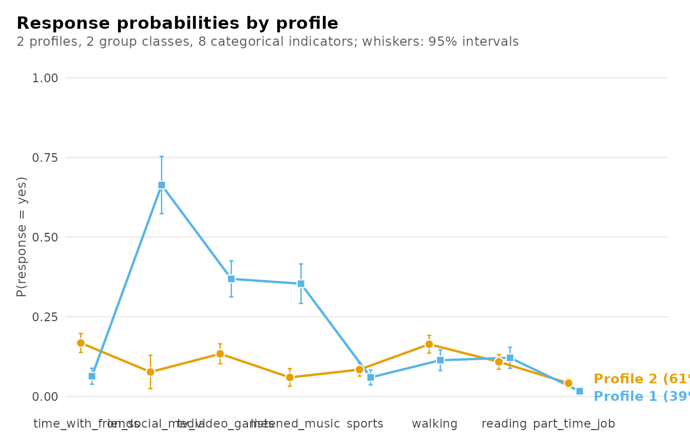
For numeric categories, such as ratings from 1 to 5, a profile plot can summarize each item’s fitted distribution on the original score scale:
plot(lca, what = "profiles")                       # probability-weighted means
plot(lca, what = "profiles", statistic = "median") # fitted medians
plot(lca, what = "profiles", statistic = "mode")   # most probable scores
Means assume meaningful spacing between category scores. The median
is the smallest score whose cumulative probability reaches 0.5; tied
modes use the smallest score. These summaries use fitted probabilities,
including in FIML models, rather than averages of cases assigned to each
class. They require numeric category labels and use the raw scale.
Confidence intervals are not computed, so these plots avoid the
parameter-inference calculation used by the response-probability plot.
In mixed models, "profiles" continues to show only
continuous indicators.
To obtain the profile probabilities of each group class, we call
get_results() with "profile_probabilities",
and to compare the classes, plot() with
what = "probabilities".
get_results(lca, "profile_probabilities")
#>   group_class profile probability group_class_probability
#> 1           1       1      0.7080                   0.483
#> 2           1       2      0.2920                   0.483
#> 3           2       1      0.0751                   0.517
#> 4           2       2      0.9249                   0.517
plot(lca, what = "probabilities")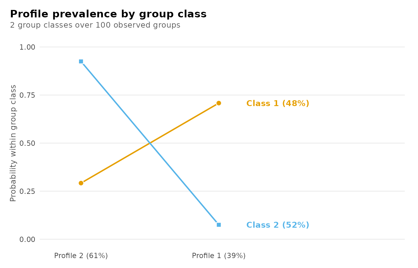
To obtain classification certainty, we call
get_results() with "entropy".
get_results(lca, "entropy")
#>         level n_classes n_units entropy_sum relative_entropy
#> 1 individuals         2    1422         411            0.583
#> 2      groups         2     100          13            0.813
Mixed indicators
To combine both kinds, we call multilpa() with all
indicators in vars and only the categorical ones in
categorical. Here three affect ratings are continuous and
the activities categorical. worried is left out: about half
its ratings are 1, which can push a profile’s variance to its lower
bound.
mixed <- multilpa(first_week,
                  vars = c("happy", "relaxed", "exhausted", activities),
                  categorical = activities, id = "student", n_profiles = 2,
                  n_group_classes = 2, n_starts = 3, seed = 1)
To obtain the means and variances of the continuous indicators, we
call get_results() on the fit; for the answer probabilities
of the categorical ones, get_results() with
"responses".
get_results(mixed)
#> No standard errors in this table: data must reproduce the original indicator data, including row order and names.
#>   profile indicator mean variance standard_deviation mean_standard_error variance_standard_error
#> 1       1     happy 3.90    1.963              1.401                  NA                      NA
#> 2       1   relaxed 3.66    1.946              1.395                  NA                      NA
#> 3       1 exhausted 4.10    2.842              1.686                  NA                      NA
#> 4       2     happy 5.98    0.659              0.812                  NA                      NA
#> 5       2   relaxed 5.77    1.016              1.008                  NA                      NA
#> 6       2 exhausted 2.32    1.976              1.406                  NA                      NA
get_results(mixed, "responses")
#> No standard errors in this table: data must reproduce the original indicator data, including row order and names.
#>    profile         indicator category probability threshold probability_standard_error
#> 1        1 time_with_friends       no      0.9309     2.601                         NA
#> 2        2 time_with_friends       no      0.8046     1.415                         NA
#> 3        1 time_with_friends      yes      0.0691        NA                         NA
#> 4        2 time_with_friends      yes      0.1954        NA                         NA
#> 5        1   on_social_media       no      0.6381     0.567                         NA
#> 6        2   on_social_media       no      0.7657     1.184                         NA
#> 7        1   on_social_media      yes      0.3619        NA                         NA
#> 8        2   on_social_media      yes      0.2343        NA                         NA
#> 9        1    tv_video_games       no      0.7370     1.030                         NA
#> 10       2    tv_video_games       no      0.8210     1.523                         NA
#> 11       1    tv_video_games      yes      0.2630        NA                         NA
#> 12       2    tv_video_games      yes      0.1790        NA                         NA
#> 13       1    listened_music       no      0.8394     1.654                         NA
#> 14       2    listened_music       no      0.8125     1.466                         NA
#> 15       1    listened_music      yes      0.1606        NA                         NA
#> 16       2    listened_music      yes      0.1875        NA                         NA
#> 17       1            sports       no      0.9385     2.726                         NA
#> 18       2            sports       no      0.9102     2.316                         NA
#> 19       1            sports      yes      0.0615        NA                         NA
#> 20       2            sports      yes      0.0898        NA                         NA
#> 21       1           walking       no      0.8821     2.012                         NA
#> 22       2           walking       no      0.8251     1.552                         NA
#> 23       1           walking      yes      0.1179        NA                         NA
#> 24       2           walking      yes      0.1749        NA                         NA
#> 25       1           reading       no      0.8670     1.874                         NA
#> 26       2           reading       no      0.9100     2.313                         NA
#> 27       1           reading      yes      0.1330        NA                         NA
#> 28       2           reading      yes      0.0900        NA                         NA
#> 29       1     part_time_job       no      0.9720     3.549                         NA
#> 30       2     part_time_job       no      0.9640     3.289                         NA
#> 31       1     part_time_job      yes      0.0280        NA                         NA
#> 32       2     part_time_job      yes      0.0360        NA                         NA
Ordinal and count indicators
The affect ratings run from 1 to 7. As categorical items
each would have six free probabilities in every profile; as
ordinal items each has six category intercepts shared by
every profile and one location per profile, which says how far up the
scale that profile sits. We pass their names as
ordinal.
affect <- c("happy", "relaxed", "worried", "exhausted")
ordinal <- multilpa(first_week, vars = c(affect, activities), id = "student",
                    ordinal = affect, categorical = activities, n_profiles = 2,
                    n_group_classes = 2, n_starts = 3, seed = 1)
ordinal
#> Two-level latent class analysis: 2 classes, 2 group classes
#> 1422 individuals in 100 groups; 8 categorical indicators
#> Also ordinal happy, relaxed, worried, exhausted (adjacent-category logit; get_results(x, "ordinal"))
#> Classes are labelled profile_1, profile_2, ... in every table.
#> Log likelihood: -13513.224891 | AIC: 27120.450 | BIC (groups): 27242.893
#> Converged: TRUE | iterations: 18 | best start: 3/3
#>
#>  profile         indicator category probability threshold
#>        1 time_with_friends       no      0.7975     1.371
#>        2 time_with_friends       no      0.9301     2.588
#>        1 time_with_friends      yes      0.2025        NA
#>        2 time_with_friends      yes      0.0699        NA
#>        1   on_social_media       no      0.7848     1.294
#>        2   on_social_media       no      0.6299     0.532
#>        1   on_social_media      yes      0.2152        NA
#>        2   on_social_media      yes      0.3701        NA
#>        1    tv_video_games       no      0.8300     1.586
#>        2    tv_video_games       no      0.7342     1.016
#>        1    tv_video_games      yes      0.1700        NA
#>        2    tv_video_games      yes      0.2658        NA
#>        1    listened_music       no      0.8104     1.452
#>        2    listened_music       no      0.8397     1.656
#>        1    listened_music      yes      0.1896        NA
#>        2    listened_music      yes      0.1603        NA
#>        1            sports       no      0.9114     2.330
#>        2            sports       no      0.9362     2.686
#>        1            sports      yes      0.0886        NA
#>        2            sports      yes      0.0638        NA
#>    ... 12 more rows.  get_results(x, "responses")
#>
#> Every other table: get_results(x, what = ), or get_results(x, "all").
get_results() with "ordinal" gives each
profile’s probability of every rating and its location.
head(get_results(ordinal, "ordinal"), 7)
#>   profile indicator category probability location location_standard_error
#> 1       1     happy        1    2.74e-05     1.86                   0.139
#> 2       1     happy        2    2.53e-04     1.86                   0.139
#> 3       1     happy        3    3.03e-03     1.86                   0.139
#> 4       1     happy        4    2.82e-02     1.86                   0.139
#> 5       1     happy        5    2.21e-01     1.86                   0.139
#> 6       1     happy        6    4.24e-01     1.86                   0.139
#> 7       1     happy        7    3.24e-01     1.86                   0.139
Indicators holding counts (number of messages sent, of absences) go
in count: each is Poisson with one mean per profile, read
with get_results(fit, "count_means"). Counts more variable
than a Poisson within a profile take
count_model = "negative_binomial", which adds a dispersion
per profile (or one shared, count_dispersion = "equal").
Both types work with membership covariates and in lta() as
well.
Reference
The calls below list other functions that work with categorical and mixed models. Each comment states what the call returns.
get_results(lca, "classification")               # class sizes and average posteriors
get_results(lca, "residuals")                    # residual association within profiles
parameter_inference(lca)                         # standard errors and intervals
enumerate_classes(first_week, vars = activities, categorical = activities,
                  id = "student", n_profiles = 2:3,
                  n_group_classes = 1:2, seed = 1)  # compare numbers of classes (slow)
plot(mixed)                                      # means of the continuous indicators
plot(mixed, what = "responses")                  # answers to the categorical ones
multilca(first_week, vars = activities, id = "student", n_profiles = 2,
         n_group_classes = 2, missing = "fiml")  # incomplete answers, if any