Latent class analysis

Fits a single-level latent class model: each observation belongs to one of n_classes unobserved classes, and within a class the discrete indicators are independent. Categorical indicators have unrestricted response probabilities; ordinal and count in ... choose the structured measurement models described by multilpa(). It is the model multilca() fits with id = NULL, and it returns the same object, so every accessor, plot and inference verb of the package applies to it. In the results the classes are labelled profile_1, profile_2, and so on, as throughout the package.

Usage

lca(data, vars, n_classes, ...)

Arguments

data

A data frame with one row per observation.

vars

Names of the discrete indicator columns. Categories are taken from the data; ordinal and count in ... identify structured discrete indicators and the remaining columns are categorical.

n_classes

Number of classes, a positive whole number.

...

Further arguments for multilca(), such as missing, n_starts, seed, min_probability and profile_covariates, except id and n_group_classes, which a single-level model does not have.

Value

A fitted multilpa object, as multilca() returns.

Details

For observations nested in groups, use multilca() with the grouping column as id, which adds latent classes of groups above the classes of observations.

Conditions

latents_bad_argument when id or n_group_classes is passed; the conditions multilca() raises otherwise.

References

Lazarsfeld, P. F., & Henry, N. W. (1968). Latent Structure Analysis. Houghton Mifflin.

See also

lpa() for continuous indicators; multilca() for the two-level model; enumerate_lca() to compare numbers of classes.

Examples

fit <- lca(student_esm, c("time_with_friends", "on_social_media",
                          "tv_video_games", "sports"),
           n_classes = 2, n_starts = 3, seed = 1)
fit
#> Latent class analysis: 2 classes
#> 2582 observations; 4 categorical indicators
#> Classes are labelled profile_1, profile_2, ... in every table.
#> Log likelihood: -4560.238322 | AIC: 9138.477 | BIC: 9191.184
#> Converged: TRUE | iterations: 96 | best start: 3/3
#> 
#>  profile         indicator category  probability  threshold
#>        1 time_with_friends       no 7.817818e-01  1.2760803
#>        2 time_with_friends       no 8.974465e-01  2.1691692
#>        1 time_with_friends      yes 2.182182e-01         NA
#>        2 time_with_friends      yes 1.025535e-01         NA
#>        1   on_social_media       no 9.999994e-01 14.3945349
#>        2   on_social_media       no 5.522218e-01  0.2096518
#>        1   on_social_media      yes 5.604446e-07         NA
#>        2   on_social_media      yes 4.477782e-01         NA
#>        1    tv_video_games       no 9.998450e-01  8.7716985
#>        2    tv_video_games       no 6.701119e-01  0.7086911
#>        1    tv_video_games      yes 1.550360e-04         NA
#>        2    tv_video_games      yes 3.298881e-01         NA
#>        1            sports       no 9.021328e-01  2.2211497
#>        2            sports       no 9.428194e-01  2.8026606
#>        1            sports      yes 9.786725e-02         NA
#>        2            sports      yes 5.718057e-02         NA
#> 
#> Every other table: get_results(x, what = ), or get_results(x, "all").
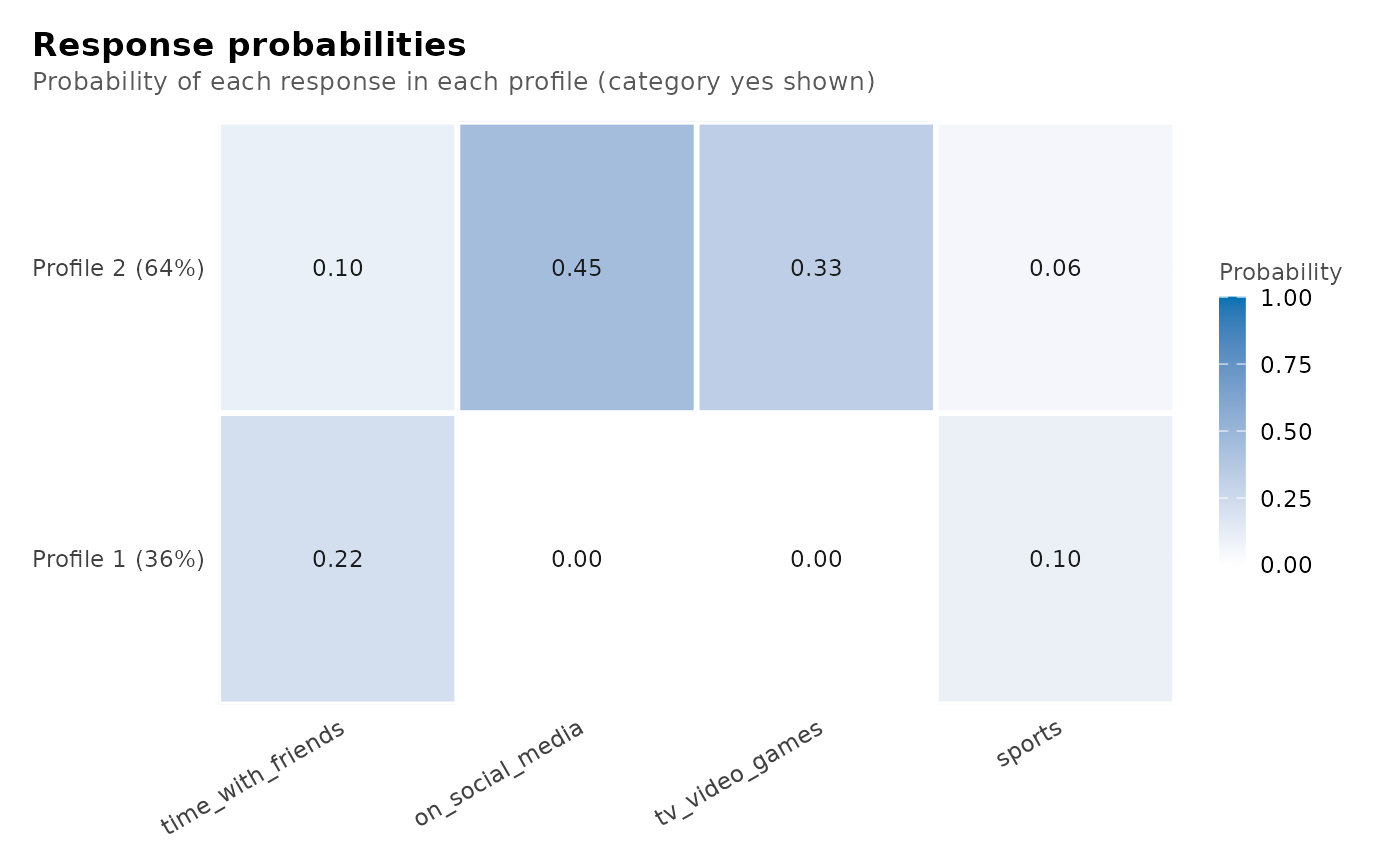
plot(fit, what = "heatmap")