Latent transition analysis

Latent transition analysis (LTA) estimates latent profiles at each occasion and the probability of moving from one profile to another between consecutive occasions. With group classes, each class has its own starting probabilities and its own transition matrix, so classes separate groups that change differently over time.

Data

course_engagement has one row per course enrolment: 1,422 enrolments from 106 students. lta() needs three kinds of variables.

Group: student identifies whose occasions belong together.
Occasion order: sequence is the position of each course in the student’s history. Students can have different numbers of occasions.
Indicators: five activity measures (browse, lectures, forum_read, forum_post, attendance), each standardized within course, so 0 is the course average.

library(latents)

Fit

To fit the model, we call lta() with vars for the indicators, id for the group, time for the occasion order, n_profiles for the number of profiles, n_group_classes for the number of group classes, n_starts for the number of random EM starts, and seed for reproducible starts.

moves <- lta(course_engagement,
             vars = c("browse", "lectures", "forum_read", "forum_post",
                      "attendance"),
             id = "student", time = "sequence",
             n_profiles = 3, n_group_classes = 2, n_starts = 3, seed = 1)
moves
#> Latent transition model: 3 profiles, 2 group classes
#> 1422 observations in 106 groups, up to 15 occasions (unbalanced, observed grid)
#> Log likelihood: -8242.967653; 47 parameters; BIC (groups): 16705.1169
#> Converged: TRUE after 84 iterations; best of 3 starts
#> 
#>  profile browse lectures forum_read forum_post attendance count proportion
#>        1 -0.776   -0.612     -0.888     -0.761     -0.929   579      0.407
#>        2  0.705    0.711      0.806      0.746      1.122   374      0.263
#>        3  0.395    0.188      0.453      0.344      0.252   469      0.330
#> 
#> Variances and standard errors: get_results(x, "profiles"). 
#> Every other table: get_results(x, what = ), or get_results(x, "all").

To check whether the starts agree, we call get_results() with "starts". Starts that reach the same log likelihood support the solution.

get_results(moves, "starts")
#>   start log_likelihood converged iterations error
#> 1     1          -8243      TRUE         84  <NA>
#> 2     2          -8243      TRUE         91  <NA>
#> 3     3          -8243      TRUE         84  <NA>

Profiles

To see the profiles, we call plot() on the fit. Each line is a profile’s mean on each indicator, and its label gives the profile’s share of the cases.

plot(moves)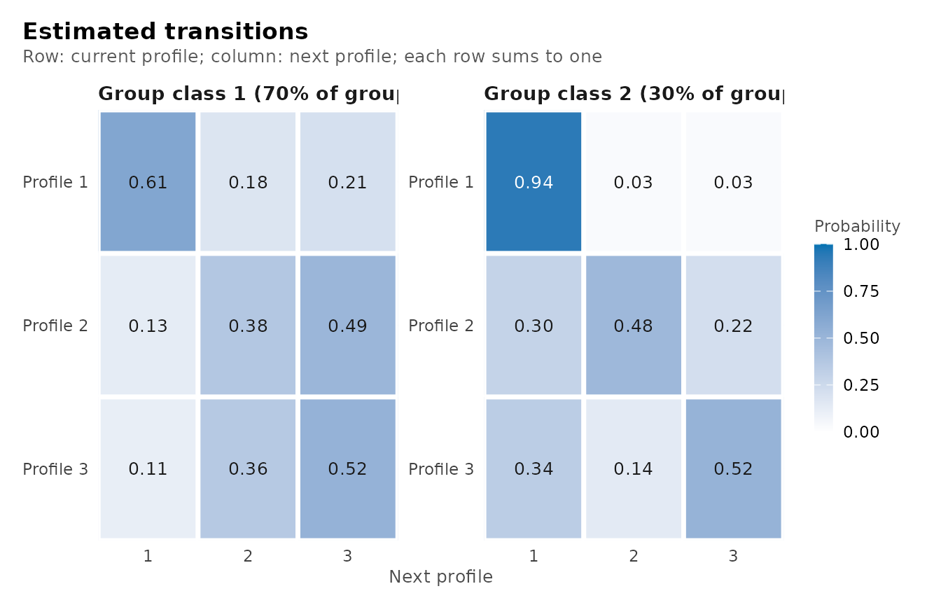

To compare profiles on a common scale, we call plot() with what = "heatmap", which shows each mean in standard deviations from the indicator’s overall mean.

plot(moves, what = "heatmap")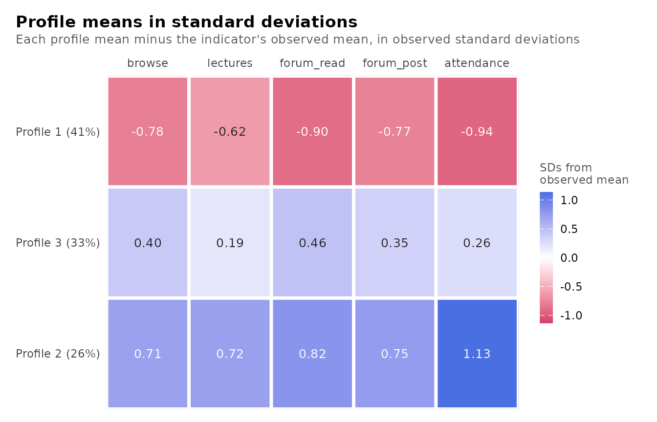

Starting probabilities

To obtain the starting probabilities, we call get_results() with "initial". probability is the chance of starting in each profile, prevalence the expected share of all occasions in it, and group_class_probability the share of groups in the class.

get_results(moves, "initial")
#>   group_class profile probability prevalence group_class_probability
#> 1           1       1    2.04e-01     0.2296                   0.699
#> 2           1       2    4.45e-01     0.3344                   0.699
#> 3           1       3    3.51e-01     0.4359                   0.699
#> 4           2       1    7.62e-01     0.8190                   0.301
#> 5           2       2    2.38e-01     0.0969                   0.301
#> 6           2       3    1.87e-05     0.0841                   0.301

Transitions

To obtain the transition probabilities, we call get_results() with "transitions". probability is the chance of moving from profile from to profile to at the next occasion, and the probabilities out of each profile sum to one. stable marks staying in the same profile, expected_count is the expected number of such moves in the data, and estimated = FALSE marks a row the data cannot inform.

get_results(moves, "transitions")
#>    group_class from to probability expected_count stable estimated group_class_probability
#> 1            1    1  1      0.6144         127.80   TRUE      TRUE                   0.699
#> 2            1    1  2      0.1763          36.67  FALSE      TRUE                   0.699
#> 3            1    1  3      0.2092          43.53  FALSE      TRUE                   0.699
#> 4            1    2  1      0.1276          38.98  FALSE      TRUE                   0.699
#> 5            1    2  2      0.3786         115.61   TRUE      TRUE                   0.699
#> 6            1    2  3      0.4938         150.81  FALSE      TRUE                   0.699
#> 7            1    3  1      0.1140          46.33  FALSE      TRUE                   0.699
#> 8            1    3  2      0.3621         147.07  FALSE      TRUE                   0.699
#> 9            1    3  3      0.5238         212.83   TRUE      TRUE                   0.699
#> 10           2    1  1      0.9385         303.35   TRUE      TRUE                   0.301
#> 11           2    1  2      0.0313          10.13  FALSE      TRUE                   0.301
#> 12           2    1  3      0.0302           9.75  FALSE      TRUE                   0.301
#> 13           2    2  1      0.2964          11.68  FALSE      TRUE                   0.301
#> 14           2    2  2      0.4823          19.01   TRUE      TRUE                   0.301
#> 15           2    2  3      0.2213           8.72  FALSE      TRUE                   0.301
#> 16           2    3  1      0.3379          11.40  FALSE      TRUE                   0.301
#> 17           2    3  2      0.1420           4.79  FALSE      TRUE                   0.301
#> 18           2    3  3      0.5200          17.54   TRUE      TRUE                   0.301

To draw the transition matrices, we call plot() with what = "transitions": one heatmap per group class, current profile in rows and next profile in columns.

plot(moves, what = "transitions")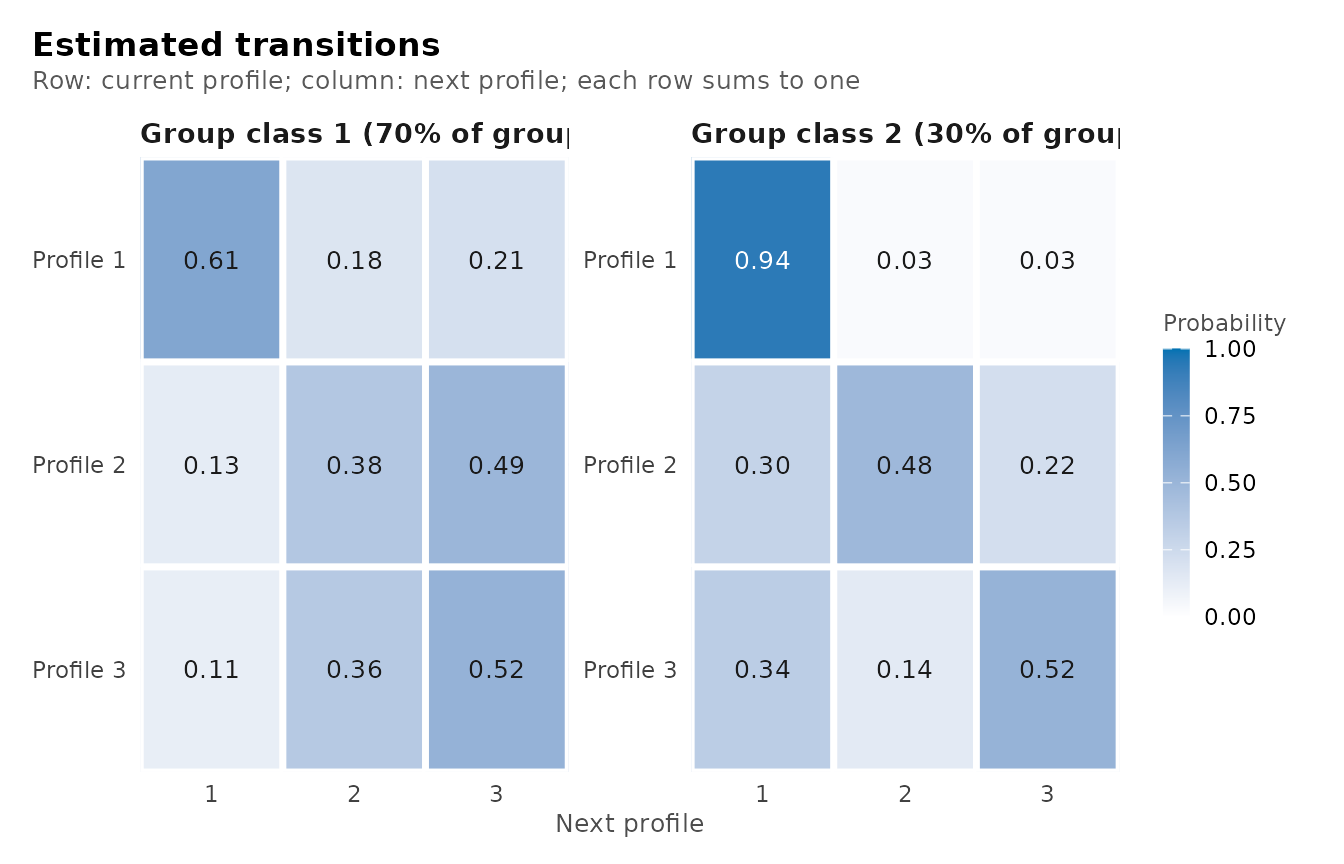

Sequences

To see each group’s path, we call plot() with what = "sequences": one row per group, coloured by its most probable profile at each occasion. These assignments ignore classification uncertainty.

plot(moves, what = "sequences")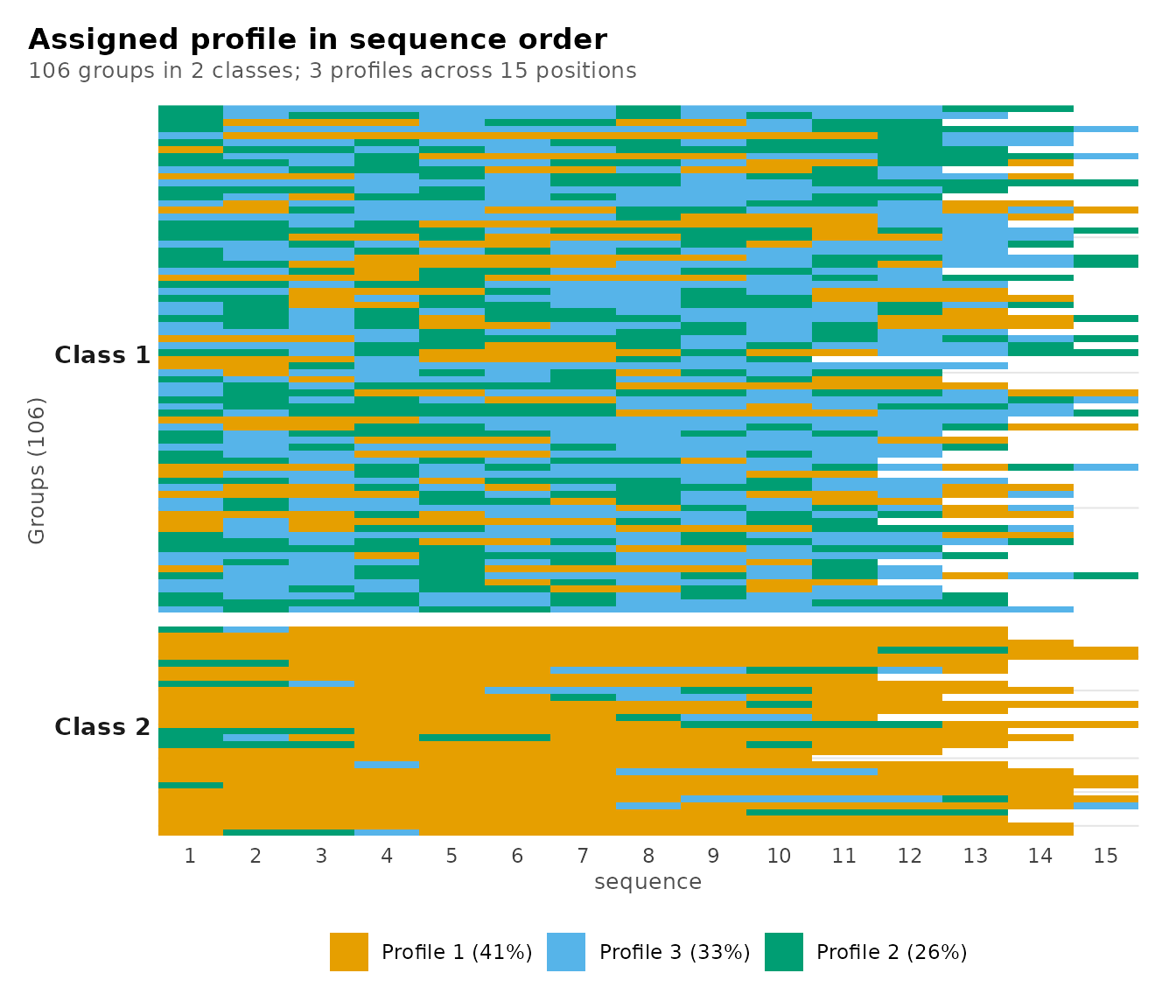

Classification

To obtain classification certainty, we call get_results() with "entropy". Relative entropy is reported for occasions and for groups: 1 means every case is assigned with certainty, 0 means no separation.

get_results(moves, "entropy")
#>         level n_classes n_units entropy_sum relative_entropy
#> 1 individuals         3    1422       309.8            0.802
#> 2      groups         2     106        16.3            0.778

To see where the uncertainty lies, we call plot() with what = "entropy" for the per-case uncertainty within each profile, and with what = "posteriors" for the posterior probability of each case’s assigned profile.

plot(moves, what = "entropy")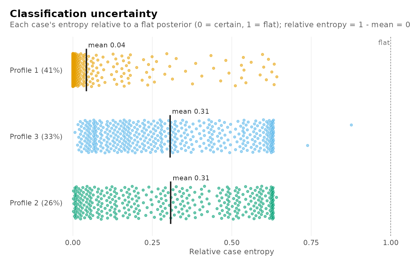

plot(moves, what = "posteriors")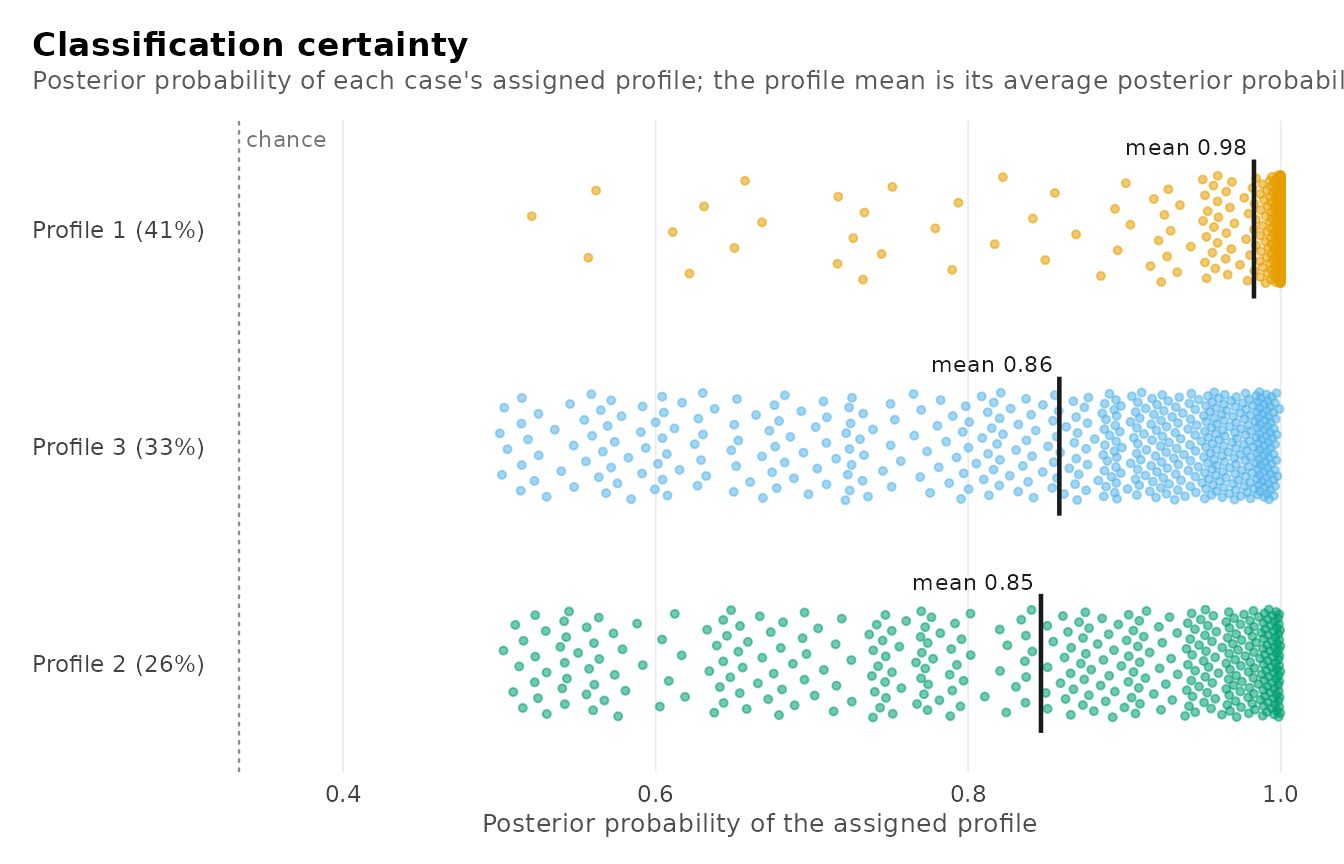

Transition networks

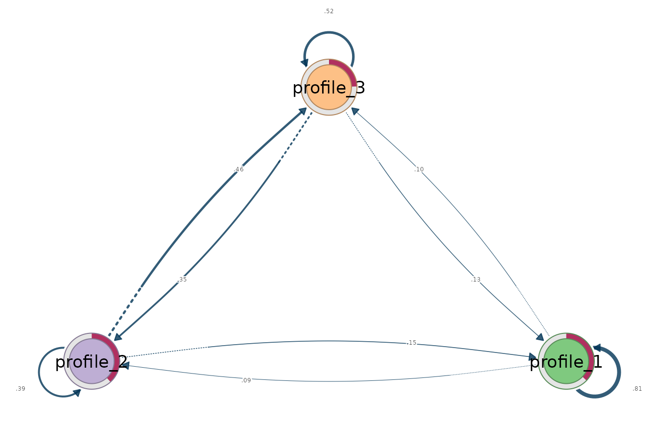
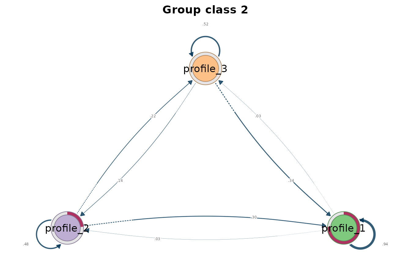
To analyse the transitions as networks, we call get_tna() for one network pooled over group classes and get_group_tna() for one network per class. Both return tna models built from the estimated transitions, which plot() draws.

plot(get_tna(moves))

plot(get_group_tna(moves))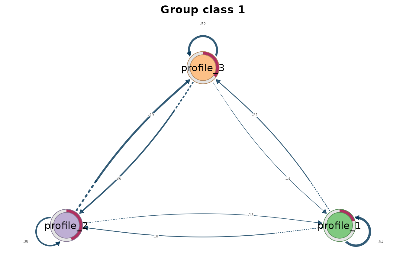

Beyond homogeneous transitions

Each default assumption of the model can be tested by relaxing it in one argument:

transition_covariates lets covariates shift the transition probabilities: the log odds of moving to each other profile rather than staying. A covariate may change over occasions.
initial_covariates lets covariates shift the starting profile.
transitions = "occasion" estimates a separate transition matrix for each move.
measurement = "occasion" lets the profiles’ means and variances differ by occasion.
order = 2 makes the next profile depend on the two previous ones.
mover_stayer = TRUE adds a class of groups that never change profile.

enumerate_classes(..., time = "sequence") compares numbers of profiles and group classes, and bootstrap_lrt() tests a model against a nested one.

Does a student’s grade in the previous course change how likely they are to move between engagement profiles? previous_grade changes from course to course:

activity <- c("browse", "lectures", "forum_read", "forum_post", "attendance")
homogeneous <- lta(course_engagement, activity, "student", n_profiles = 2,
                   time = "sequence", seed = 1)
grade <- lta(course_engagement, activity, "student", n_profiles = 2,
             time = "sequence", transition_covariates = "previous_grade",
             seed = 1)
get_results(grade, "transition_coefficients")
#>     group_class      from        to           term estimate standard_error statistic  p_value
#> 1 group_class_1 profile_1 profile_2    (Intercept)  -1.4634          0.130   -11.257 2.14e-29
#> 2 group_class_1 profile_1 profile_2 previous_grade   0.0440          0.130     0.339 7.35e-01
#> 3 group_class_1 profile_2 profile_1    (Intercept)  -1.8402          0.118   -15.566 1.25e-54
#> 4 group_class_1 profile_2 profile_1 previous_grade   0.0342          0.121     0.283 7.77e-01
#>   conf_low conf_high odds_ratio
#> 1   -1.718    -1.209      0.231
#> 2   -0.211     0.299      1.045
#> 3   -2.072    -1.608      0.159
#> 4   -0.202     0.271      1.035

The grade’s odds ratios are close to one and their intervals include one: in these data, the previous grade does not change the chance of switching profile. A second-order chain, where the next profile depends on the two previous ones, does not earn its extra parameters either:

second <- lta(course_engagement, activity, "student", n_profiles = 2,
              time = "sequence", order = 2, seed = 1)
BIC(homogeneous, grade, second)
#>             df   BIC
#> homogeneous 23 16778
#> grade       25 16787
#> second      27 16786

These extensions return a fit with transition and initial logit coefficients, Wald standard errors and probabilities per occasion; they were checked against Mplus, depmixS4 and LMest.

Assumptions

By default the next profile depends only on the current profile and the group class, and transition probabilities are the same at every occasion; the arguments above relax each of these.
Profiles have the same definition at every occasion unless measurement = "occasion".
Indicators are independent within a profile (the default diagonal covariance; covariance_model = "full" or model = relaxes it).

Written by Mohammed Saqr and Sonsoles López-Pernas