Multilevel latent profile analysis

Multilevel latent profile analysis (MLPA) estimates latent profiles at the observation level and, at a higher level, identifies latent group classes that differ in how probable each profile is for their observations. Each profile is characterized by a mean and variance for each indicator and is defined identically across all group classes. The group classes therefore differ only in the probabilities associated with the profiles.

Data

course_engagement has one row per course enrolment: 1,422 enrolments from 106 students. multilpa() needs two kinds of variables.

Group: student identifies which enrolments belong to the same student.
Indicators: five activity measures (browse, lectures, forum_read, forum_post, attendance), each standardized within course, so 0 is the course average.

The data are simulated, and two further variables record the structure that generated them: engagement for each enrolment and student_type for each student.

library(latents)

Clustering within groups

To check how much each indicator varies between groups, we call descriptives() with vars for the indicators and id for the group. icc is the share of an indicator’s variance that lies between groups.

descriptives(course_engagement,
             vars = c("browse", "lectures", "forum_read", "forum_post",
                      "attendance"),
             id = "student")
#>     variable    n n_missing      mean    sd   min  max n_distinct n_groups    icc
#> 1     browse 1422         0 -2.81e-05 0.989 -3.14 2.49        398      106 0.1923
#> 2   lectures 1422         0 -4.22e-05 0.989 -2.91 3.22        399      106 0.0878
#> 3 forum_read 1422         0  7.03e-05 0.989 -2.73 2.81        400      106 0.2240
#> 4 forum_post 1422         0 -2.11e-05 0.989 -2.61 3.10        397      106 0.1503
#> 5 attendance 1422         0  7.74e-05 0.989 -2.45 2.41        401      106 0.2215

Fit

To fit the model, we call multilpa() with vars for the indicators, id for the group, n_profiles for the number of profiles, n_group_classes for the number of group classes, n_starts for the number of random EM starts, and seed for reproducible starts. Printing the fit gives the profile means.

fit <- multilpa(course_engagement,
                vars = c("browse", "lectures", "forum_read", "forum_post",
                         "attendance"),
                id = "student", n_profiles = 2, n_group_classes = 2,
                n_starts = 10, seed = 1)
fit
#> Two-level latent profile analysis: 2 profiles, 2 group classes
#> 1422 individuals in 106 groups; varying diagonal residual covariance (VVI)
#> Log likelihood: -8439.816424 | AIC: 16925.633 | BIC (groups): 16986.892
#> Converged: TRUE | iterations: 9 | best start: 1/10
#> 
#>  profile browse lectures forum_read forum_post attendance count proportion
#>        1  0.540    0.427      0.620      0.530      0.649   834      0.587
#>        2 -0.766   -0.606     -0.879     -0.753     -0.921   588      0.413
#> 
#> Variances and standard errors: get_results(x, "profiles"). 
#> Every other table: get_results(x, what = ), or get_results(x, "all").

To check whether the starts agree, we call get_results() with "starts". Starts that reach the same log likelihood support the solution.

get_results(fit, "starts")
#>    start log_likelihood converged iterations error boundary
#> 1      1          -8440      TRUE          9  <NA>    FALSE
#> 2      2          -8440      TRUE         12  <NA>    FALSE
#> 3      3          -8440      TRUE          9  <NA>    FALSE
#> 4      4          -8440      TRUE         12  <NA>    FALSE
#> 5      5          -8440      TRUE          9  <NA>    FALSE
#> 6      6          -8440      TRUE         12  <NA>    FALSE
#> 7      7          -8440      TRUE          9  <NA>    FALSE
#> 8      8          -8440      TRUE         12  <NA>    FALSE
#> 9      9          -8440      TRUE          9  <NA>    FALSE
#> 10    10          -8440      TRUE          9  <NA>    FALSE

Profiles

To obtain the profile means and variances, we call get_results() on the fit. There is one row per profile and indicator.

get_results(fit)
#>    profile  indicator   mean variance standard_deviation mean_standard_error
#> 1        1     browse  0.540    0.590              0.768              0.0271
#> 2        1   lectures  0.427    0.845              0.919              0.0325
#> 3        1 forum_read  0.620    0.481              0.694              0.0247
#> 4        1 forum_post  0.530    0.689              0.830              0.0295
#> 5        1 attendance  0.649    0.384              0.620              0.0223
#> 6        2     browse -0.766    0.528              0.727              0.0312
#> 7        2   lectures -0.606    0.538              0.734              0.0309
#> 8        2 forum_read -0.879    0.363              0.603              0.0262
#> 9        2 forum_post -0.753    0.421              0.649              0.0277
#> 10       2 attendance -0.921    0.374              0.611              0.0264
#>    variance_standard_error
#> 1                   0.0295
#> 2                   0.0421
#> 3                   0.0244
#> 4                   0.0348
#> 5                   0.0196
#> 6                   0.0322
#> 7                   0.0321
#> 8                   0.0228
#> 9                   0.0261
#> 10                  0.0228

To see the profiles, we call plot() on the fit. Each line is a profile’s mean on each indicator, and its label gives the profile’s share of the cases.

plot(fit)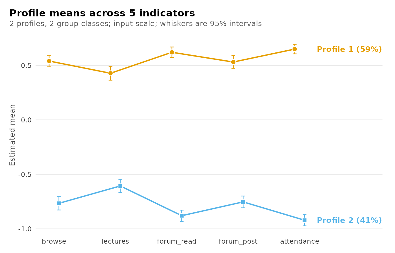

Group classes

To obtain the profile probabilities of each group class, we call get_results() with "profile_probabilities". probability is the chance that an observation of a group in that class falls in each profile, and group_class_probability is the share of groups in the class.

get_results(fit, "profile_probabilities")
#>   group_class profile probability group_class_probability
#> 1           1       1       0.786                   0.675
#> 2           1       2       0.214                   0.675
#> 3           2       1       0.170                   0.325
#> 4           2       2       0.830                   0.325

To compare the group classes, we call plot() with what = "probabilities": one line per group class across the profiles.

plot(fit, what = "probabilities")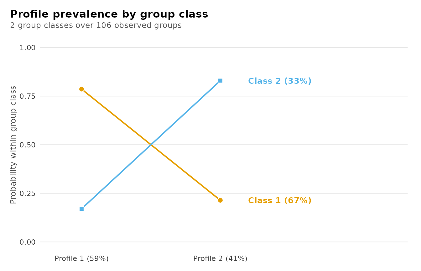

Class sizes

To obtain class sizes, we call get_results() with "counts". effective_count sums the posterior probabilities, so it need not be a whole number.

get_results(fit, "counts")
#>         level class effective_count effective_proportion
#> 1 individuals     1           834.1                0.587
#> 2 individuals     2           587.9                0.413
#> 3      groups     1            71.5                0.675
#> 4      groups     2            34.5                0.325

Classification

To obtain classification certainty, we call get_results() with "entropy". Relative entropy is reported for observations and for groups: 1 means every case is assigned with certainty, 0 means no separation.

get_results(fit, "entropy")
#>         level n_classes n_units entropy_sum relative_entropy
#> 1 individuals         2    1422       60.94            0.938
#> 2      groups         2     106        4.43            0.940

To add each observation’s assigned profile and group class to the data, we call get_results() with "assignments" and data for the data frame. It returns the data in its original row order with five added columns: profile and group_class hold the most probable classes, uncertainty is one minus the posterior probability of the assigned profile, and the posterior_profile_ columns hold the posterior probability of each profile. Assignment takes the most probable class, so profile and group_class alone ignore classification uncertainty.

get_results(fit, "assignments", data = course_engagement) |> head()
#>   student course sequence browse lectures forum_read forum_post attendance previous_grade
#> 1       1     23        1   0.73    -0.08       0.30       0.67       0.72           0.54
#> 2       1     19        2   0.68     0.53      -0.02      -0.55       0.70          -0.71
#> 3       1      4        3  -1.51    -0.51      -0.91      -0.80      -0.97           1.98
#> 4       1     18        4   0.64    -1.02      -1.62      -1.20      -1.26          -1.42
#> 5       1     16        5  -0.94    -0.37      -0.71      -0.28      -1.52          -0.67
#> 6       1     29        6  -0.36    -0.46      -0.77      -0.43      -1.34          -0.40
#>   engagement student_type profile group_class uncertainty posterior_profile_1 posterior_profile_2
#> 1    engaged     wavering       1           2    4.44e-04            1.00e+00            0.000444
#> 2    engaged     wavering       1           2    1.49e-02            9.85e-01            0.014854
#> 3 disengaged     wavering       2           2    2.42e-06            2.42e-06            0.999998
#> 4 disengaged     wavering       2           2    3.86e-06            3.86e-06            0.999996
#> 5 disengaged     wavering       2           2    5.75e-06            5.75e-06            0.999994
#> 6 disengaged     wavering       2           2    2.28e-05            2.28e-05            0.999977

Recovery of the known structure

To compare the fitted classes with known labels, we call get_results() with "assignments", data for the data frame, and truth for the columns that hold the labels. engagement is compared with the profiles and student_type with the group classes. Class numbers are arbitrary, so the table is read by its largest cells.

get_results(fit, "assignments", data = course_engagement,
            truth = c("engagement", "student_type"))
#>    assignment class        truth      value   n proportion
#> 1     profile     1   engagement disengaged  16     0.0274
#> 2     profile     2   engagement disengaged 569     0.9726
#> 3     profile     1   engagement    engaged 820     0.9797
#> 4     profile     2   engagement    engaged  17     0.0203
#> 5 group_class     1 student_type  committed  61     0.9839
#> 6 group_class     2 student_type  committed   1     0.0161
#> 7 group_class     1 student_type   wavering  10     0.2273
#> 8 group_class     2 student_type   wavering  34     0.7727

Reference

The calls below list the other tables, functions and views available for a fitted model. Each comment states what the call returns.

# Tables: get_results(fit, what)
get_results(fit, "all")                          # every table, as a named list
get_results(fit, "covariances")                  # within-profile residual covariances
get_results(fit, "posteriors")                   # one row per observation and profile
get_results(fit, "posteriors", format = "wide")  # one row per observation
get_results(fit, "group_posteriors")             # one row per group and group class
get_results(fit, "classification")               # class sizes and average posteriors
get_results(fit, "average_posteriors")           # mean posterior by assigned class
get_results(fit, "classification_errors")        # P(assigned class | true class)
get_results(fit, "bch_weights")                  # weights for three-step analysis
get_results(fit, "residuals")                    # residual correlations within profiles
get_results(fit, "information_criteria")         # AIC, BIC and the other criteria
get_results(fit, "model")                        # one row describing the fit
get_results(fit, "data")                         # the variables used in the fit
as.data.frame(fit)                               # the profile table

# Summaries and diagnostics
descriptives(fit)                    # indicator summaries with the ICC
descriptives(fit, by = "profile")    # the same, by assigned profile
diagnostics(fit)                     # every classification diagnostic
report(fit)                          # summary, diagnostics and plots together

# Inference and likelihood
parameter_inference(fit)             # standard errors and Wald intervals
confint(fit)                         # confidence intervals
vcov(fit)                            # covariance matrix of the estimates
logLik(fit)                          # log likelihood
AIC(fit)                             # Akaike information criterion
BIC(fit)                             # BIC with the number of groups
nobs(fit)                            # number of groups

# Plots: plot(fit, what)
plot_views()                # every view and what it shows
plot(fit, what = "bars")             # profile means with 95% intervals
plot(fit, what = "heatmap")          # means in standard deviations
plot(fit, what = "sizes")            # effective size of each profile
plot(fit, what = "entropy")          # per-case classification uncertainty
plot(fit, what = "posteriors")       # posterior of each assigned profile
plot(fit, what = "avepp")            # average posteriors, assigned by posterior class
plot(fit, what = "all")              # every view this fit supports

# Other functions
sensitivity(fit, seeds = 1:10)       # refits under several seeds
starting_values(fit)                 # parameters to start another fit

The evaluation vignette covers enumerate_classes(), candidate_fit() and bootstrap_lrt(); the covariates vignette covers three_step(), r3step() and fit_staged(); the transitions vignette covers lta(), get_tna() and get_group_tna().

Sampling weights

When students were sampled unequally, for example wavering students at half the rate of committed ones, each student carries a sampling weight, and the fit should estimate the population rather than the sample. We pass the weight column as weights. The weight belongs to the independent unit, here the student, so it must be constant within id. The fit maximizes the weighted (pseudo) log likelihood, with the weights scaled to sum to the number of students, and reports Kish’s effective sample size.

weighted_data <- transform(course_engagement,
                           survey_weight = ifelse(student_type == "wavering", 2, 1))
weighted_fit <- multilpa(weighted_data,
                         vars = c("browse", "lectures", "forum_read",
                                  "forum_post", "attendance"),
                         id = "student", n_profiles = 2, n_group_classes = 2,
                         weights = "survey_weight", n_starts = 10, seed = 1)
weighted_fit
#> Two-level latent profile analysis: 2 profiles, 2 group classes
#> 1422 individuals in 106 groups; varying diagonal residual covariance (VVI)
#> Sampling weights `survey_weight` (pseudo maximum likelihood): Kish effective n 94.5 of 106 units
#> Log likelihood: -8341.125778 | AIC: 16728.252 | BIC (groups): 16789.511
#> Converged: TRUE | iterations: 9 | best start: 1/10
#> 
#>  profile browse lectures forum_read forum_post attendance count proportion
#>        1  0.525    0.446      0.605      0.515      0.655   701      0.495
#>        2 -0.770   -0.608     -0.877     -0.742     -0.921   715      0.505
#> 
#> Variances and standard errors: get_results(x, "profiles"). 
#> Every other table: get_results(x, what = ), or get_results(x, "all").

Under weights the inverse information is not the variance of the estimates, so parameter_inference() reports sandwich standard errors by default and refuses vcov_type = "observed".

head(parameter_inference(weighted_fit), 4)
#>         level   outcome       term parameter estimate standard_error statistic   p_value p_adjusted
#> 1 measurement profile_1     browse      mean    0.525         0.0323      16.3  1.76e-59   1.76e-59
#> 2 measurement profile_1   lectures      mean    0.446         0.0365      12.2  2.23e-34   2.23e-34
#> 3 measurement profile_1 forum_read      mean    0.605         0.0263      23.0 6.60e-117  6.60e-117
#> 4 measurement profile_1 forum_post      mean    0.515         0.0317      16.2  2.72e-59   2.72e-59
#>   conf_low conf_high
#> 1    0.462     0.589
#> 2    0.375     0.518
#> 3    0.553     0.656
#> 4    0.453     0.578

lta(), mixture_regression() and every family of multilpa() take weights the same way. The bootstrap likelihood ratio test does not: it simulates from the model, not from the sampling design.

All tables

To see every table at once, we call summary() on the fit, with rows for the number of rows shown per table.

print(summary(fit), rows = 3)
#> Multilevel LPA: 2 profiles and 2 group classes
#> Individuals: 1422; groups: 106; parameters: 23; converged: TRUE
#> Log likelihood: -8439.816424; AIC: 16925.633
#> BIC (groups): 16986.892; BIC (individuals): 17046.609
#> Best likelihood replicated in 10/10 starts (absolute tolerance 0.00844).
#> 
#> -- profiles --------------------------------------------------------
#>  profile  indicator   mean variance standard_deviation mean_standard_error variance_standard_error
#>        1     browse 0.5396   0.5899             0.7680             0.02710                 0.02948
#>        1   lectures 0.4274   0.8447             0.9191             0.03249                 0.04210
#>        1 forum_read 0.6198   0.4815             0.6939             0.02473                 0.02440
#>    ... 7 more rows.  get_results(x, what = "profiles")
#> 
#> -- responses -------------------------------------------------------
#>    (no rows)
#> 
#> -- covariances -----------------------------------------------------
#>  profile  indicator indicator_2 covariance
#>        1     browse      browse     0.5899
#>        1   lectures      browse     0.0000
#>        1 forum_read      browse     0.0000
#>    ... 47 more rows.  get_results(x, what = "covariances")
#> 
#> -- profile_probabilities -------------------------------------------
#>  group_class profile probability group_class_probability
#>            1       1      0.7859                  0.6747
#>            1       2      0.2141                  0.6747
#>            2       1      0.1705                  0.3253
#>    ... 1 more rows.  get_results(x, what = "profile_probabilities")
#> 
#> -- counts ----------------------------------------------------------
#>        level class effective_count effective_proportion
#>  individuals     1          834.10               0.5866
#>  individuals     2          587.90               0.4134
#>       groups     1           71.52               0.6747
#>    ... 1 more rows.  get_results(x, what = "counts")
#> 
#> -- posteriors ------------------------------------------------------
#>  row group profile posterior modal
#>    1     1       1 9.996e-01  TRUE
#>    2     1       1 9.851e-01  TRUE
#>    3     1       1 2.421e-06 FALSE
#>    ... 2841 more rows.  get_results(x, what = "posteriors")
#> 
#> -- group_posteriors ------------------------------------------------
#>  group group_size log_likelihood group_class posterior modal
#>      1         13         -61.52           1 1.473e-05 FALSE
#>      2         13         -71.94           1 6.391e-08 FALSE
#>      3         14         -76.69           1 1.000e+00  TRUE
#>    ... 209 more rows.  get_results(x, what = "group_posteriors")
#> 
#> -- assignments -----------------------------------------------------
#>  student browse lectures forum_read forum_post attendance profile group_class uncertainty
#>        1   0.73    -0.08       0.30       0.67       0.72       1           2   4.436e-04
#>        1   0.68     0.53      -0.02      -0.55       0.70       1           2   1.485e-02
#>        1  -1.51    -0.51      -0.91      -0.80      -0.97       2           2   2.421e-06
#>  posterior_profile_1 posterior_profile_2
#>            9.996e-01           0.0004436
#>            9.851e-01           0.0148536
#>            2.421e-06           0.9999976
#>    ... 1419 more rows.  get_results(x, what = "assignments")
#> 
#> -- classification --------------------------------------------------
#>        level class n_modal proportion_modal estimated_n estimated_proportion average_posterior
#>  individuals     1     836           0.5879      834.10               0.5866            0.9849
#>  individuals     2     586           0.4121      587.90               0.4134            0.9818
#>       groups     1      71           0.6698       71.52               0.6747            0.9920
#>  odds_correct_classification
#>                        46.08
#>                        76.35
#>                        59.89
#>    ... 1 more rows.  get_results(x, what = "classification")
#> 
#> -- average_posteriors ----------------------------------------------
#>        level assigned_class class n_assigned average_posterior
#>  individuals              1     1        836           0.98493
#>  individuals              1     2        836           0.01507
#>  individuals              2     1        586           0.01824
#>    ... 5 more rows.  get_results(x, what = "average_posteriors")
#> 
#> -- classification_errors -------------------------------------------
#>        level true_class assigned_class probability
#>  individuals          1              1     0.98718
#>  individuals          1              2     0.01282
#>  individuals          2              1     0.02142
#>    ... 5 more rows.  get_results(x, what = "classification_errors")
#> 
#> -- bch_weights -----------------------------------------------------
#>        level unit assigned_class class   weight
#>  individuals    1              1     1  1.01327
#>  individuals    1              1     2 -0.01327
#>  individuals    2              1     1  1.01327
#>    ... 3053 more rows.  get_results(x, what = "bch_weights")
#> 
#> -- entropy ---------------------------------------------------------
#>        level n_classes n_units entropy_sum relative_entropy
#>  individuals         2    1422      60.940           0.9382
#>       groups         2     106       4.435           0.9396
#> 
#> -- residuals -------------------------------------------------------
#>    profile indicator_1 indicator_2     kind observed expected residual effective_n statistic df
#>  profile_1    lectures  attendance gaussian   0.2339        0   0.2339       834.1     6.871 NA
#>  profile_2  forum_read  attendance gaussian   0.2287        0   0.2287       587.9     5.630 NA
#>  profile_1  forum_read  attendance gaussian   0.2088        0   0.2088       834.1     6.109 NA
#>    p_value p_adjusted
#>  6.374e-12  6.374e-12
#>  1.799e-08  1.799e-08
#>  1.001e-09  1.001e-09
#>    ... 17 more rows.  get_results(x, what = "residuals")
#> 
#> -- information_criteria --------------------------------------------
#>  log_likelihood n_parameters   aic   kic bic_groups bic_individual sabic_groups sabic_individual
#>           -8440           23 16926 16952      16987          17047        16914            16974
#>  caic_groups caic_individual awe_groups awe_individual icl_groups icl_individual clc_groups
#>        17010           17070      17172          17404      16996          17168      16889
#>  clc_individual
#>           17002
#> 
#> -- model -----------------------------------------------------------
#>  n_observations n_informative n_groups n_profiles n_group_classes centering covariance_structure
#>            1422          1422      106          2               2      none                  VVI
#>  n_parameters n_parameters_with_measurement log_likelihood   aic bic_groups bic_individual
#>            23                            23          -8440 16926      16987          17047
#>  converged iterations boundary small_classes best_start n_best_replicated weights
#>       TRUE          9    FALSE         FALSE          1                10    <NA>
#> 
#> -- stages ----------------------------------------------------------
#>  stage group_classes fixed log_likelihood parameters parameters_with_measurement converged
#>  joint             2  <NA>          -8440         23                          23      TRUE
#> 
#> -- starts ----------------------------------------------------------
#>  start log_likelihood converged iterations error boundary
#>      1          -8440      TRUE          9  <NA>    FALSE
#>      2          -8440      TRUE         12  <NA>    FALSE
#>      3          -8440      TRUE          9  <NA>    FALSE
#>    ... 7 more rows.  get_results(x, what = "starts")
#> 
#> -- data ------------------------------------------------------------
#>  student browse lectures forum_read forum_post attendance
#>        1   0.73    -0.08       0.30       0.67       0.72
#>        1   0.68     0.53      -0.02      -0.55       0.70
#>        1  -1.51    -0.51      -0.91      -0.80      -0.97
#>    ... 1419 more rows.  get_results(x, what = "data")
#> 
#> 19 tables above, truncated to fit. get_results(x, what = ) returns any
#> of them whole, and get_results(x, what = "all") returns every one.

Assumptions

Profiles have the same means and variances in every group class.
Observations are independent given their group’s class, and groups are independent of one another.
Indicators are independent within a profile (the default diagonal covariance; covariance_model = "full" relaxes it).
The numbers of profiles and group classes are chosen by the analyst; see the evaluation vignette for comparing them.

Written by Mohammed Saqr and Sonsoles López-Pernas