Case study: Multilevel latent profile analysis of course engagement

Multilevel latent profile analysis (MLPA) is used when observations are nested within higher-level units and the aim is to identify latent profiles at the observation level while also describing how the prevalence of those profiles varies across units. Examples include repeated measurements nested within persons, students nested within schools, patients nested within clinics, or employees nested within organizations. Because observations from the same higher-level unit may be dependent, MLPA extends standard latent profile analysis by modeling the data at two levels. Latent profiles are defined at Level 1, whereas latent classes at Level 2 describe differences between higher-level units in the composition of those profiles.

Consider a repeated-measures application. A person may occupy different profiles on different occasions. Let $C_{it}$ denote the profile of person $i$ at occasion $t$ , and let $G_i$ denote the person’s Level-2 latent class. The model estimates the conditional probability $P(C_{it}=k\mid G_i=m)$ that an observation belongs to profile $k$ given that the person belongs to class $m$ . In this way, MLPA separates variation across repeated observations from variation between persons in the profiles they tend to occupy.

This distinction is also central to VaSSTra (López-Pernas & Saqr, 2023), which separates state diversity from person heterogeneity using a sequential estimation strategy. VaSSTra first establishes a common state space across all observations and then summarizes each person’s repeated observations within that space. MLPA takes a different approach: the observation-level profiles and person-level classes are estimated jointly within a single model. Both approaches allow the same person to occupy several states across repeated observations, but they differ in how the states and the person-level representation are constructed.

The latents package fits MLPA models using maximum likelihood with multiple expectation-maximization starting values. In this vignette, we work through a three-profile, three-student-class example using longitudinal data on course engagement. The focus is on specifying, estimating, and interpreting the model. The companion guides cover model evaluation, covariates and staged estimation, and latent transitions.

library(latents)

Longitudinal course engagement

The engagement example revisits the setting studied by Saqr and López-Pernas (2021), The longitudinal trajectories of online engagement over a full program. The study distinguished three engagement states within courses and three longer-term student trajectories. Here, we use the bundled synthetic course_engagement data to reproduce the same type of nested longitudinal design. The purpose of the example is to illustrate the analytical questions and workflow; the estimates reported below apply only to the synthetic package data.

Each row represents one student’s enrolment in one course. Enrolments are therefore the Level-1 observations, while students are the Level-2 units within which those observations are nested. A student who takes several courses appears on several rows. The variable student identifies the Level-2 unit, course identifies the course associated with each enrolment, and sequence records the position of that course in the student’s observed history. Students need not contribute the same number of enrolments. The MLPA model accounts for the grouping of enrolments within students; it does not include a separate course-level random effect or latent structure.

Five activity indicators describe the student’s engagement during each enrolment. The indicators are simulated on the log1p(count) scale and standardized within course. Each value can therefore be interpreted as the enrolment’s distance from the mean of that particular course, expressed in course-specific standard deviations. A value above zero indicates more activity than the course average, whereas a value below zero indicates less activity than the course average.

This within-course standardization is important for the interpretation of the profiles. Raw activity volumes can differ substantially across courses because of differences in course design, duration, or expected workload. The indicators therefore describe a student’s engagement relative to other students taking the same course rather than relative to the cohort as a whole. The profiles identified below are therefore recurring patterns of relative engagement within courses.

Variable	Definition
`browse`	Course page views.
`lectures`	Lecture videos viewed.
`forum_read`	Forum posts read.
`forum_post`	Forum posts written.
`attendance`	Days active in the course.
`previous_grade`	Standardized grade from the preceding course, with an entry grade at the first course.

The indicator vector vars selects the five measures used to define engagement profiles. Identifiers and previous_grade stay outside the measurement model. The package accepts a character vector of column names.

vars <- c("browse", "lectures", "forum_read", "forum_post", "attendance")

Descriptive statistics and clustering within students

The descriptives() function summarizes the distributions of the activity indicators and estimates their intraclass correlations (ICCs), using student as the grouping variable. The ICC describes how much of the variation in an indicator is attributable to differences between students rather than variation across enrolments within the same student. It is defined as

$\mathrm{ICC} = \frac{\sigma^2_{\mathrm{between}}} {\sigma^2_{\mathrm{between}}+\sigma^2_{\mathrm{within}}}.$

Here, $\sigma^2_{\mathrm{between}}$ is the variance between students and $\sigma^2_{\mathrm{within}}$ is the variance across enrolments within students.

An ICC near zero indicates little between-student variation in an indicator’s average level, whereas an ICC near one indicates little variation across enrolments within students. With the one-way random-effects estimator used here, an estimated ICC can occasionally be negative because of sampling variation; such estimates are generally interpreted as indicating little or no detectable between-student clustering for that indicator.

ICCs describe the clustering of each activity indicator separately. They do not determine how many Level-1 profiles or Level-2 student classes should be fitted. In particular, students may differ in the composition of their engagement profiles even when their average levels on the individual indicators are similar. The ICCs are therefore descriptive measures of the multilevel structure in the observed indicators.

The descriptive table reports means, standard deviations, ranges, and ICCs for the activity indicators, together with sample sizes and missingness.

descriptives(course_engagement, vars = vars, id = "student")

#>     variable    n n_missing       mean     sd   min  max n_distinct n_groups     icc
#> 1     browse 1422         0 -2.813e-05 0.9891 -3.14 2.49        398      106 0.19229
#> 2   lectures 1422         0 -4.219e-05 0.9889 -2.91 3.22        399      106 0.08779
#> 3 forum_read 1422         0  7.032e-05 0.9890 -2.73 2.81        400      106 0.22403
#> 4 forum_post 1422         0 -2.110e-05 0.9890 -2.61 3.10        397      106 0.15035
#> 5 attendance 1422         0  7.736e-05 0.9889 -2.45 2.41        401      106 0.22145

The data comprise 1,422 enrolments from 106 students, with complete observations on all activity indicators. Because the indicators were standardized within course, their pooled means are approximately zero and their standard deviations are close to one. The estimated ICCs range from 0.088 for lectures to 0.224 for forum_read: about 9% to 22% of the variance in the individual indicators is attributable to differences between students. Most variation therefore occurs across enrolments within students, while a meaningful share reflects between-student differences. This combination of within- and between-student variation is the structure that the multilevel model is designed to represent.

Three engagement profiles and three student classes

The multilpa() function estimates engagement profiles from the five activity indicators and student classes from the distribution of those profiles across each student’s enrolments. A 3 × 3 model contains three Level-1 enrolment profiles and three Level-2 student classes. Each student class is characterized by a different set of probabilities for the three enrolment profiles, while an individual student may contribute enrolments to more than one profile.

Each engagement profile is defined by a mean and variance for every activity indicator. These profile-specific parameters are shared across student classes. Thus, a given profile represents the same pattern of engagement regardless of which student class it occurs in. What differs across student classes is the relative frequency with which their enrolments occupy the profiles.

The conditional profile probabilities introduced above can be written as

$\pi_{k\mid m}=P(C_{it}=k\mid G_i=m),$

where $\pi_{k\mid m}$ is the probability that an enrolment belongs to profile $k$ when the student belongs to class $m$ . For each student class, these probabilities range from zero to one and sum to one across the three profiles. The Level-2 class probability

$\omega_m=P(G_i=m)$

gives the proportion of students represented by class $m$ .

The model relies on several distributional and independence assumptions. Within each profile, the activity indicators are modeled as Gaussian, and the same profile definitions apply to all students. Students are treated as independent Level-2 units, and enrolments within a student are conditionally independent given the student’s latent class. With the default diagonal covariance structure, the activity indicators are additionally assumed to be independent within each profile. Substantial residual associations between indicators after accounting for profile membership may indicate that this assumption is too restrictive and can affect the resulting profile solution.

The 3 × 3 model considered here is one candidate representation of the latent structure. The evaluation vignette shows how this model can be compared with alternatives containing different numbers of Level-1 profiles and Level-2 student classes.

The model is estimated from ten random starts to check whether different initial values lead to the same likelihood solution. Setting seed = 1 makes these starts reproducible while restoring the caller’s random state after estimation. A tighter convergence criterion, specified through tol, is used to support the subsequent calculation of standard errors. The argument time = "sequence" retains the order of each student’s courses so that enrolment histories can be displayed in sequence. Course order does not enter the present model, however: the model describes the composition of profiles across a student’s enrolments. Transitions between successive profiles are addressed by the separate longitudinal model.

fit <- multilpa(course_engagement, vars, id = "student", time = "sequence",
                n_profiles = 3, n_group_classes = 3, n_starts = 10,
                max_iter = 2000, tol = 1e-10, seed = 1)

Profile means

Printing the fitted model gives a compact summary of the Level-1 profile solution. Each row represents one engagement profile and reports its estimated mean on each activity indicator, together with its estimated enrolment membership.

fit

#> Two-level latent profile analysis: 3 profiles, 3 group classes
#> 1422 individuals in 106 groups; varying diagonal residual covariance (VVI)
#> Log likelihood: -8348.428704 | AIC: 16772.857 | BIC (groups): 16874.068
#> Converged: TRUE | iterations: 42 | best start: 1/10
#> 
#>  profile  browse lectures forum_read forum_post attendance count proportion
#>        1  0.3870   0.1856     0.4464     0.3376     0.2564   478     0.3362
#>        2 -0.7768  -0.6123    -0.8914    -0.7623    -0.9400   575     0.4043
#>        3  0.7089   0.7135     0.8109     0.7503     1.1328   369     0.2595
#> 
#> Variances and standard errors: get_results(x, "profiles"). 
#> Every other table: get_results(x, what = ), or get_results(x, "all").

Profile 1 has the highest estimated mean on all five activity indicators, profile 2 has intermediate means, and profile 3 has the lowest means. For attendance, the profile means are 1.133, 0.256, and -0.940 standard deviations from the corresponding course mean. For browse, they are 0.709, 0.387, and -0.777. The profiles therefore primarily distinguish different levels of recorded activity, although the separation varies across indicators. For example, the difference between profiles 1 and 2 is substantially larger for attendance than for browse.

Profile numbers are arbitrary labels assigned during estimation and have no inherent substantive meaning. In this fitted model, we refer to profiles 1, 2, and 3 as higher activity, intermediate activity, and lower activity, respectively. The numbering may change when the model is fitted again or when a different specification is estimated. Profile labels should therefore be based on the estimated indicator means rather than on the profile numbers themselves.

Profile and class sizes

The get_results() function extracts result tables from the fitted model. The "counts" table reports effective membership at both levels: the estimated number of enrolments in each Level-1 profile and the estimated number of students in each Level-2 class. Effective membership is obtained by summing posterior membership probabilities rather than assigning each case to its single most likely profile or class. For example, a student with a posterior probability of 0.80 of belonging to class 2 contributes 0.80 to the effective size of that class. Because these probabilities are summed across enrolments or students, the resulting counts need not be whole numbers. Counts based on assigning each case to its most likely profile or class, by contrast, would always be integers.

get_results(fit, "counts")

#>         level class effective_count effective_proportion
#> 1 individuals     1          478.03               0.3362
#> 2 individuals     2          574.96               0.4043
#> 3 individuals     3          369.01               0.2595
#> 4      groups     1           27.65               0.2609
#> 5      groups     2           31.03               0.2927
#> 6      groups     3           47.32               0.4464

The lower-activity profile has the largest effective membership, accounting for 575.0 enrolments, or 40.4% of the total. The higher-activity profile accounts for 369.2 enrolments, or 26.0%. At Level 2, student class 2 is the largest, with an effective membership of 47.3 students, corresponding to 44.6% of the sample. Classes 1 and 3 have effective memberships of 27.7 and 31.0 students, respectively.

How students differ in their profile composition

The "profile_probabilities" table shows how the three enrolment profiles are distributed within each student class. For each class, it reports the probability of an enrolment belonging to each Level-1 profile, together with the prevalence of that Level-2 class among students. Each row therefore answers two related questions: which profiles characterize students in this class, and how common is the class in the student population?

get_results(fit, "profile_probabilities")

#>   group_class profile probability group_class_probability
#> 1           1       1     0.54695                  0.2609
#> 2           1       2     0.05523                  0.2609
#> 3           1       3     0.39782                  0.2609
#> 4           2       1     0.07013                  0.2927
#> 5           2       2     0.84667                  0.2927
#> 6           2       3     0.08320                  0.2927
#> 7           3       1     0.38811                  0.4464
#> 8           3       2     0.31716                  0.4464
#> 9           3       3     0.29472                  0.4464

Student class 1 is characterized mainly by the higher-activity and intermediate-activity profiles. Conditional on membership in class 1, the probabilities of an enrolment occupying profiles 1, 2, and 3 are 0.398, 0.547, and 0.055, respectively. Student class 2 has a more balanced profile composition, with corresponding probabilities of 0.295, 0.388, and 0.317. Student class 3 is strongly characterized by the lower-activity profile: an enrolment from a student in this class has a probability of 0.847 of occupying profile 3. The estimated prevalences of student classes 1, 2, and 3 are 0.261, 0.446, and 0.293, respectively.

The probability plot provides a visual comparison of these class-specific profile compositions on a common scale from zero to one. Each line represents a student class, and each point shows the conditional probability of an enrolment occupying a particular profile within that class. Differences in the shape of the lines therefore show how the distribution of engagement profiles varies across student classes.

plot(fit, what = "probabilities")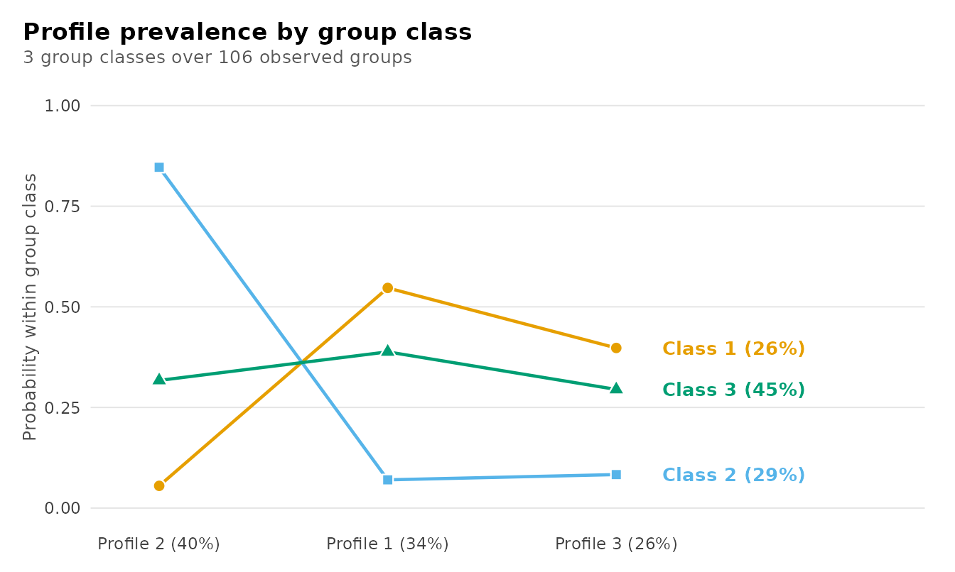

Class 2 has an almost level profile because its probabilities are similar across the three engagement profiles. In contrast, class 3 rises sharply to 0.847 for the lower-activity profile, whereas class 1 falls to 0.055 for that same profile. These differences illustrate how student classes can have distinct profile compositions even though students within each class may still occupy more than one engagement profile across their enrolments.

Checking the estimation

The "starts" table reports the final log likelihood, convergence status, and variance-boundary status for each random start. Agreement across starts provides evidence that the estimation is repeatedly reaching the same solution, although it does not establish that this solution is the global maximum.

get_results(fit, "starts")

#>    start log_likelihood converged iterations error boundary
#> 1      1          -8348      TRUE         42  <NA>    FALSE
#> 2      2          -8348      TRUE         33  <NA>    FALSE
#> 3      3          -8348      TRUE         42  <NA>    FALSE
#> 4      4          -8348      TRUE         39  <NA>    FALSE
#> 5      5          -8348      TRUE         33  <NA>    FALSE
#> 6      6          -8348      TRUE         33  <NA>    FALSE
#> 7      7          -8348      TRUE         33  <NA>    FALSE
#> 8      8          -8348      TRUE         42  <NA>    FALSE
#> 9      9          -8348      TRUE         42  <NA>    FALSE
#> 10    10          -8348      TRUE         42  <NA>    FALSE

All ten starts converge to a log likelihood of approximately -8348.4, and none has an active variance bound. The identical likelihoods across starts indicate that the fitted solution is stable with respect to the starting values used in this analysis.

Profile means as a plot

plot() displays the estimated profile means across the five activity indicators. Because the indicators were standardized within course, the vertical axis is expressed in standard deviations from the corresponding course mean. Line types and point symbols distinguish the profiles in addition to colour.

plot(fit, subtitle = "Profile means, standard deviations from each course mean")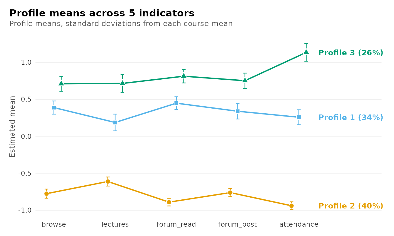

The three profiles retain the same ordering across all five indicators, with profile 1 highest, profile 2 intermediate, and profile 3 lowest. The distance between profiles 1 and 2 varies across indicators: they are relatively close on page browsing but more clearly separated on attendance, consistent with the estimated means reported above. Because the profiles differ mainly in overall elevation rather than in the shape of their indicator patterns, the principal contrast is the overall amount of recorded activity.

Reading each student’s course history

The "sequences" table arranges each student’s enrolments in course order and shows the profile assigned to each enrolment. Assignment is based on the profile with the highest posterior probability, so these sequences provide a simplified summary of the fitted model and do not represent classification uncertainty. In the wide format, each row corresponds to a student and successive observed courses appear in columns.

get_results(fit, "sequences", format = "wide") |> head(4)

#>   group group_class sequence_1 sequence_2 sequence_3 sequence_4 sequence_5 sequence_6
#> 1     1           2          1          1          2          2          2          2
#> 2     2           2          2          2          2          2          2          2
#> 3     3           1          3          1          1          1          1          1
#> 4     4           1          3          1          3          3          1          1
#>   sequence_7 sequence_8 sequence_9 sequence_10 sequence_11 sequence_12 sequence_13
#> 1          2          2          2           2           2           2           2
#> 2          2          2          2           2           2           2           2
#> 3          1          3          1           1           1           1           3
#> 4          1          3          1           3           1           1           1
#>   sequence_14 sequence_15
#> 1        <NA>        <NA>
#> 2        <NA>        <NA>
#> 3           3        <NA>
#> 4        <NA>        <NA>

Students 1 and 2 are assigned to student class 3. Student 1 is assigned to the intermediate-activity profile for the first two observed courses and to the lower-activity profile for the courses that follow, whereas student 2 is assigned to the lower-activity profile throughout the observed sequence. Students 3 and 4 are assigned to class 1 and have enrolments classified as both higher activity and intermediate activity. These patterns illustrate the class-specific profile compositions described above, but they should not be interpreted as estimated transition processes. Trailing NA values indicate courses that were not observed for that student rather than missing profile assignments within the observed history.

The "sequence_summary" table summarizes the modal student-class assignments and the amount of longitudinal information available within each class. It reports the number of students, enrolments, and observed courses in each assigned class. The gaps column counts students with an unobserved occasion between observed occasions in their sequence; simply having a shorter observed history does not constitute a gap.

get_results(fit, "sequence_summary")

#>   group_class groups observations mean_length median_length shortest longest complete gaps
#> 1           1     25          330       13.20          13.0       11      15        4    0
#> 2           2     30          403       13.43          13.5       10      15        7    0
#> 3           3     51          689       13.51          14.0       10      15       13    0

The modal assignments place 25, 51, and 30 students in classes 1, 2, and 3, respectively. Their mean sequence lengths are 13.20, 13.51, and 13.43 observed courses. Thus, the classes have similar amounts of longitudinal information, even though their profile compositions differ substantially. None of the observed sequences contains an internal gap.

Interpretation

Profile composition and profile order describe different aspects of the data. Two students may spend similar proportions of their enrolments in the same profiles while encountering those profiles in a different sequence. The MLPA estimated here captures the former by modeling class-specific profile probabilities, but it does not model the ordering of profiles over time. The transition vignette extends the analysis to that question by estimating probabilities of moving from one profile to another across successive observations.

Limitations

The bundled data are designed to reproduce the structure of the published case for instructional purposes; they do not provide a numerical replication of the original study. The published analysis used latent class analysis followed by hidden Markov modeling, whereas the present example fits a joint MLPA model. The resulting three student classes therefore summarize differences in profile composition across enrolments rather than reproducing the longitudinal trajectories estimated in the original study.

The 3 × 3 specification should also be treated as a candidate model rather than a definitive representation of the latent structure. Its adequacy depends on comparisons with alternative numbers of Level-1 profiles and Level-2 classes, as well as on the model’s distributional assumptions. In particular, the default diagonal covariance structure assumes that the activity indicators are conditionally independent within each profile. Residual associations among the indicators may violate this assumption and alter the estimated profile solution. In addition, modal profile and class assignments simplify the fitted model by ignoring classification uncertainty. The evaluation vignette examines these issues using the same data and candidate specification.

References

López-Pernas, S., & Saqr, M. (2023). From variables to states to trajectories (VaSSTra): A method for modelling the longitudinal dynamics of learning and behaviour. In Proceedings TEEM 2022: Tenth International Conference on Technological Ecosystems for Enhancing Multiculturality (pp. 1169-1178). Springer Nature Singapore. doi:10.1007/978-981-99-0942-1_123.

Saqr, M., & López-Pernas, S. (2021). The longitudinal trajectories of online engagement over a full program. Computers & Education, 175, 104325. doi:10.1016/j.compedu.2021.104325.

Written by Mohammed Saqr and Sonsoles López-Pernas