Case study: Latent transition analysis of course engagement

Latent transition analysis (LTA) estimates the probability of moving from one latent profile to another between consecutive occasions (Collins & Lanza, 2010). With group classes, each class has its own starting distribution and its own transition matrix, so the classes separate students who differ in how their engagement changes from students who differ only in where it starts.

Data and model

course_engagement holds 1,422 course enrolments of 106 students, ordered within each student by sequence. The five indicators are simulated on the log1p scale of activity counts and standardized within course. The data are synthetic and revisit the design of Saqr and López-Pernas (2021), who asked how students’ online engagement develops across a program. That study identified course-level engagement states and longer-term trajectories with latent class analysis and hidden Markov models. Here, three profiles and two student classes are working choices for illustrating the transition model; they do not establish the number of profiles or reproduce the published estimates.

For student $i$ at course position $t$ , $C_{it}$ is the latent profile and $G_i$ the student’s class. The model estimates

the initial probabilities $\delta_{k\mid m}=P(C_{i1}=k\mid G_i=m)$ ,
the transition probabilities $a_{kl\mid m}=P(C_{i,t+1}=l\mid C_{it}=k,G_i=m)$ , which sum to one across destinations $l$ ,
and a Gaussian mean and variance for each profile and indicator.

The transitions are first order and homogeneous: the next profile depends only on the current profile and the student’s class, and the probabilities are the same at every position. Profile means and variances are shared across positions and classes, so a change of profile is a change of state. Indicators are independent within a profile under the default diagonal covariance. The fit can fail to reach the global maximum from a single start, and a transition that is rare within a class is estimated from little information; the expected count of each transition shows how much.

library(latents)
vars <- c("browse", "lectures", "forum_read", "forum_post", "attendance")

moves <- lta(course_engagement, vars, "student", n_profiles = 3,
             n_group_classes = 2, time = "sequence", n_starts = 10, seed = 1)
get_results(moves, "starts")
#>    start log_likelihood converged iterations error
#> 1      1          -8243      TRUE         84  <NA>
#> 2      2          -8243      TRUE         91  <NA>
#> 3      3          -8243      TRUE         84  <NA>
#> 4      4          -8243      TRUE        121  <NA>
#> 5      5          -8243      TRUE         72  <NA>
#> 6      6          -8243      TRUE        258  <NA>
#> 7      7          -8243      TRUE         96  <NA>
#> 8      8          -8243      TRUE        104  <NA>
#> 9      9          -8243      TRUE         88  <NA>
#> 10    10          -8243      TRUE         97  <NA>

All ten starts converge to the same log likelihood, so the solution is replicated within this seed’s starts.

The profiles

plot() draws the profile means across the indicators, with point size showing profile prevalence.

plot(moves)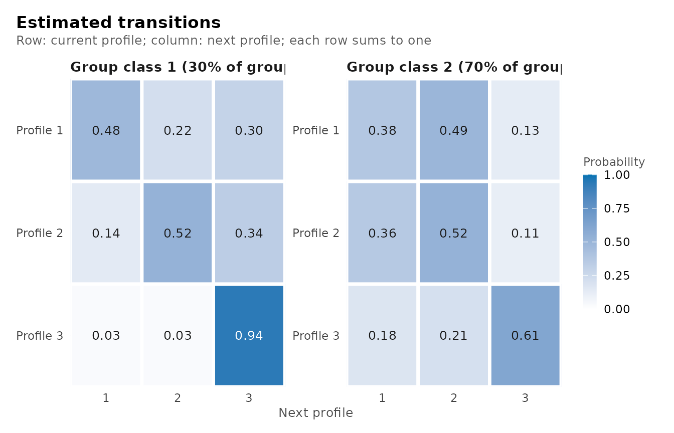

get_results(moves)
#> No standard errors in this table: Wald inference is unavailable when a probability sits at its lower bound: its logit is at minus infinity, where the likelihood has no curvature to invert.
#>    profile  indicator    mean variance standard_deviation mean_standard_error
#> 1        1     browse  0.7052   0.5295             0.7276                  NA
#> 2        1   lectures  0.7108   0.7966             0.8925                  NA
#> 3        1 forum_read  0.8064   0.4652             0.6821                  NA
#> 4        1 forum_post  0.7464   0.5772             0.7598                  NA
#> 5        1 attendance  1.1225   0.2071             0.4551                  NA
#> 6        2     browse  0.3955   0.6100             0.7810                  NA
#> 7        2   lectures  0.1883   0.7590             0.8712                  NA
#> 8        2 forum_read  0.4535   0.4578             0.6766                  NA
#> 9        2 forum_post  0.3439   0.7145             0.8453                  NA
#> 10       2 attendance  0.2526   0.2041             0.4518                  NA
#> 11       3     browse -0.7760   0.5149             0.7175                  NA
#> 12       3   lectures -0.6117   0.5417             0.7360                  NA
#> 13       3 forum_read -0.8881   0.3540             0.5950                  NA
#> 14       3 forum_post -0.7607   0.4149             0.6441                  NA
#> 15       3 attendance -0.9293   0.3727             0.6105                  NA
#>    variance_standard_error
#> 1                       NA
#> 2                       NA
#> 3                       NA
#> 4                       NA
#> 5                       NA
#> 6                       NA
#> 7                       NA
#> 8                       NA
#> 9                       NA
#> 10                      NA
#> 11                      NA
#> 12                      NA
#> 13                      NA
#> 14                      NA
#> 15                      NA

Profile 1 is the lowest on every indicator, profile 2 the highest, and profile 3 lies between them; their attendance means are -0.929, 1.122 and 0.252. The profiles are therefore lower, higher and intermediate activity. The heatmap shows the same means as standard deviations from each indicator’s grand mean.

plot(moves, what = "heatmap")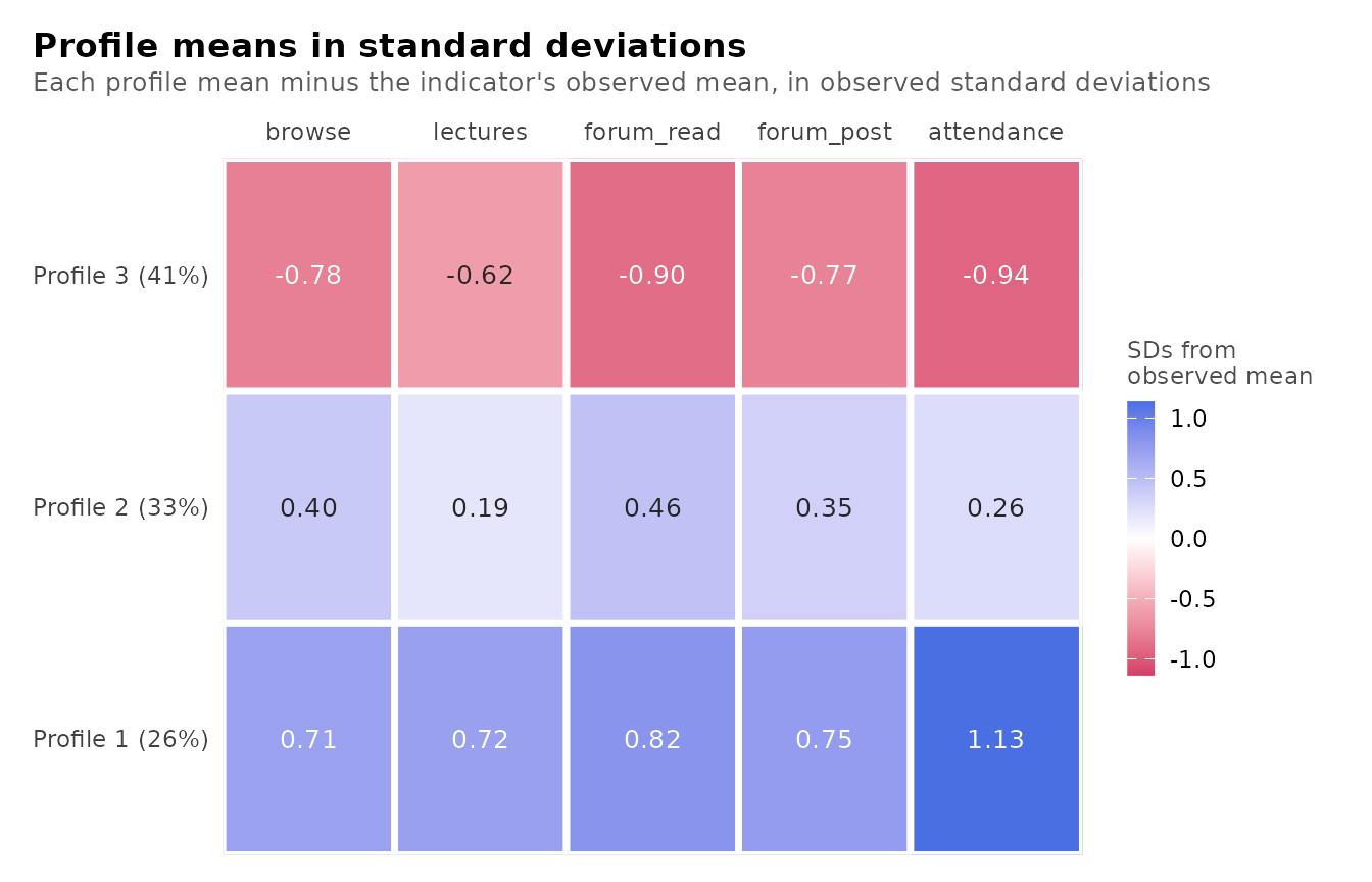

The contrast between profiles is present on all five indicators, so the profiles differ in overall activity more than in its composition.

Where students start

In the "initial" table, probability is $\delta_{k\mid m}$ , the chance of starting in each profile. prevalence is the expected share of all of a class’s enrolments in that profile, across the whole history, and group_class_probability is the share of students in the class.

get_results(moves, "initial")
#>   group_class profile probability prevalence group_class_probability
#> 1           1       1   2.379e-01    0.09687                  0.3008
#> 2           1       2   5.810e-07    0.08438                  0.3008
#> 3           1       3   7.621e-01    0.81875                  0.3008
#> 4           2       1   4.451e-01    0.33432                  0.6992
#> 5           2       2   3.515e-01    0.43608                  0.6992
#> 6           2       3   2.034e-01    0.22960                  0.6992

Student class 1, with 30.1% of students, starts in the lower-activity profile with probability 0.762 and in the higher-activity profile with probability 0.238; its probability of starting in the intermediate profile is effectively zero. Class 2, with 69.9% of students, starts across all three profiles, with probabilities 0.204, 0.445 and 0.351. Starting and overall shares differ: class 1 starts in the lower profile with probability 0.762, but 0.819 of its enrolments are expected there over the whole history, while class 2 starts in the higher profile with probability 0.445 and spends 0.334 of its enrolments there.

How engagement changes

The "transitions" table gives $a_{kl\mid m}$ for every class and pair of profiles. stable marks staying in the same profile. expected_count is the posterior expected number of such transitions in the data, so it can be fractional, and it shows how much information supports each estimate. estimated = FALSE would mark a row the data cannot inform, because the profile is never occupied before a student’s last course; such a row holds uniform placeholder values. Every row is estimated in this fit.

get_results(moves, "transitions")
#>    group_class from to probability expected_count stable estimated group_class_probability
#> 1            1    1  1     0.48240         19.013   TRUE      TRUE                  0.3008
#> 2            1    1  2     0.22079          8.706  FALSE      TRUE                  0.3008
#> 3            1    1  3     0.29682         11.697  FALSE      TRUE                  0.3008
#> 4            1    2  1     0.14153          4.791  FALSE      TRUE                  0.3008
#> 5            1    2  2     0.52228         17.676   TRUE      TRUE                  0.3008
#> 6            1    2  3     0.33619         11.393  FALSE      TRUE                  0.3008
#> 7            1    3  1     0.03129         10.117  FALSE      TRUE                  0.3008
#> 8            1    3  2     0.03023          9.771  FALSE      TRUE                  0.3008
#> 9            1    3  3     0.93848        303.412   TRUE      TRUE                  0.3008
#> 10           2    1  1     0.37840        115.475   TRUE      TRUE                  0.6992
#> 11           2    1  2     0.49402        150.794  FALSE      TRUE                  0.6992
#> 12           2    1  3     0.12758         38.942  FALSE      TRUE                  0.6992
#> 13           2    2  1     0.36203        147.047  FALSE      TRUE                  0.6992
#> 14           2    2  2     0.52388        212.879   TRUE      TRUE                  0.6992
#> 15           2    2  3     0.11409         46.351  FALSE      TRUE                  0.6992
#> 16           2    3  1     0.17632         36.654  FALSE      TRUE                  0.6992
#> 17           2    3  2     0.20932         43.531  FALSE      TRUE                  0.6992
#> 18           2    3  3     0.61436        127.751   TRUE      TRUE                  0.6992

The transition plot draws each class’s matrix as a heatmap, with the origin profile in rows and the destination in columns.

plot(moves, what = "transitions")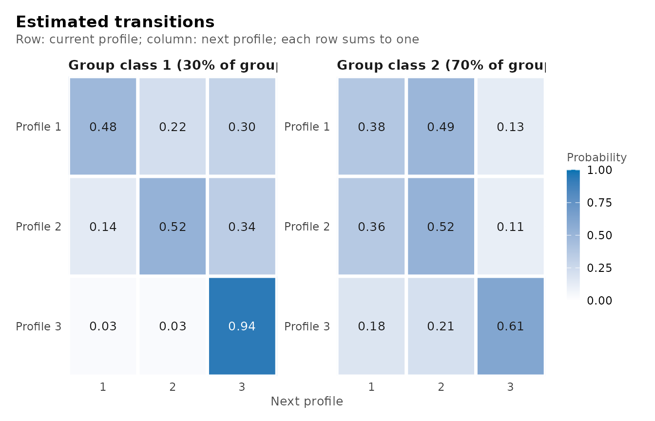

In class 1, lower activity persists with probability 0.938, estimated from 303 expected transitions. Each of its other transitions rests on fewer than 20 expected transitions, because class-1 students rarely leave the lower profile. Class 2 moves between profiles. Its students remain in the lower profile with probability 0.614, move from higher to intermediate activity with probability 0.494, and from intermediate to higher with probability 0.362. Class 1 is therefore a persistently low-engagement class, and class 2 a class whose engagement changes from course to course.

Sparse and boundary estimates

Some estimates rest on very little information. Class 1’s probability of starting in the intermediate profile is at its lower bound, because no class-1 student is expected to start there. Class 1’s transitions out of the higher and intermediate profiles rest on between 4.8 and 19.0 expected transitions each, because its students rarely leave the lower profile. A probability near zero shows that the data carry little information about that movement, not that the movement is impossible. Estimates like these can also mean that the chosen number of classes divides the available transitions too finely.

Assigned sequences

The sequence plot shows each student’s modal profile at each course position, one row per student. Modal assignment discards classification uncertainty.

plot(moves, what = "sequences")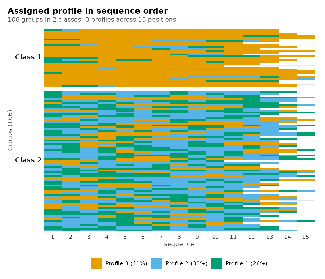

get_results(moves, "sequence_summary")
#>   group_class groups observations mean_length median_length shortest longest complete gaps
#> 1           1     31          417       13.45            13       10      15        8    0
#> 2           2     75         1005       13.40            14       10      15       16    0

The summary gives the number of students and courses in each assigned class. Sequence lengths differ between students, so the rows of the plot end at different positions.

Classification uncertainty

get_results(moves, "entropy")
#>         level n_classes n_units entropy_sum relative_entropy
#> 1 individuals         3    1422      309.75           0.8017
#> 2      groups         2     106       16.37           0.7772

Relative entropy is 0.802 for enrolments and 0.777 for students. The entropy plot shows, within each profile, how the per-case entropy contributions are distributed, and the posterior plot shows the posterior probability of each case’s assigned profile.

plot(moves, what = "entropy")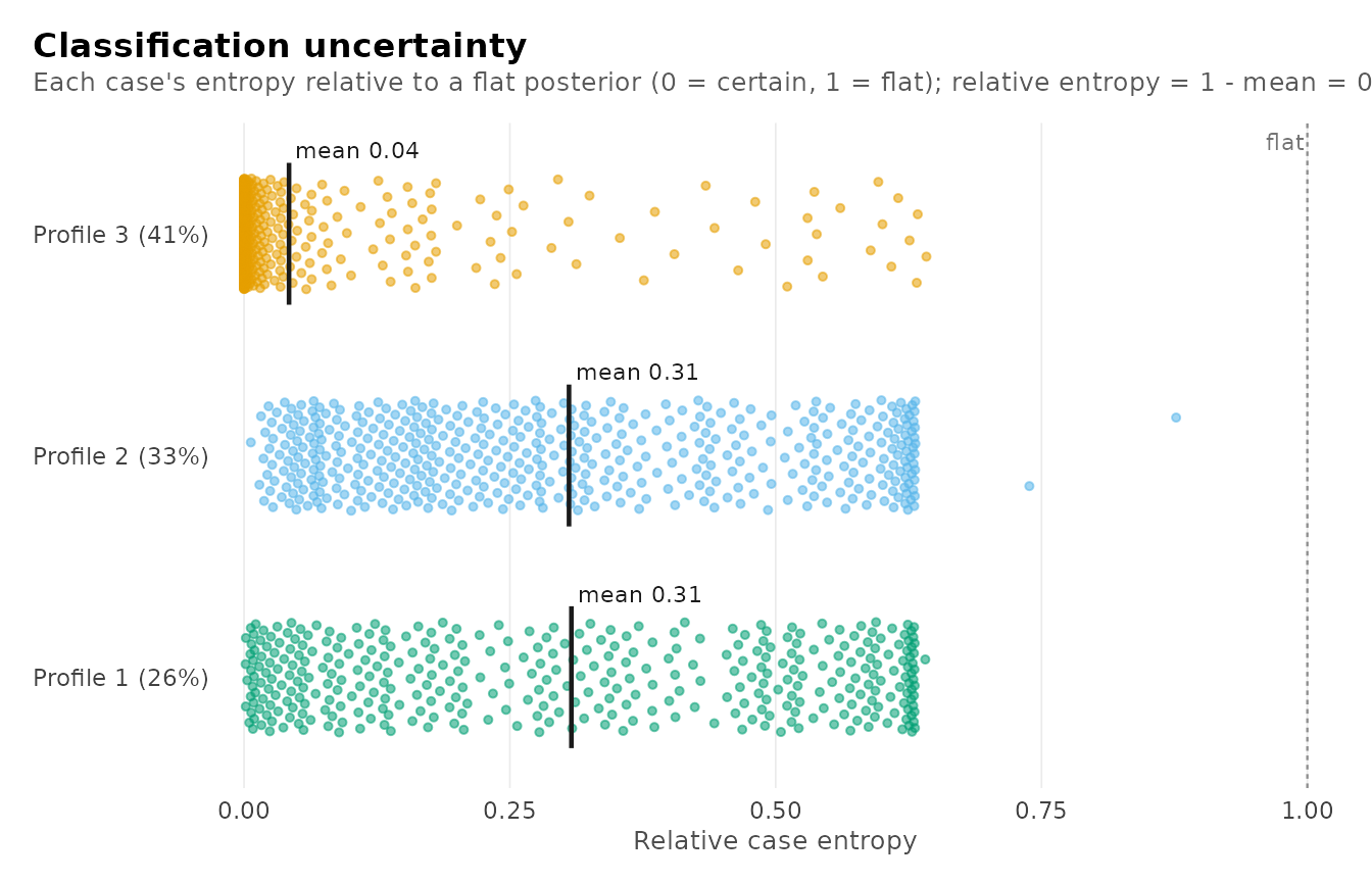

plot(moves, what = "posteriors")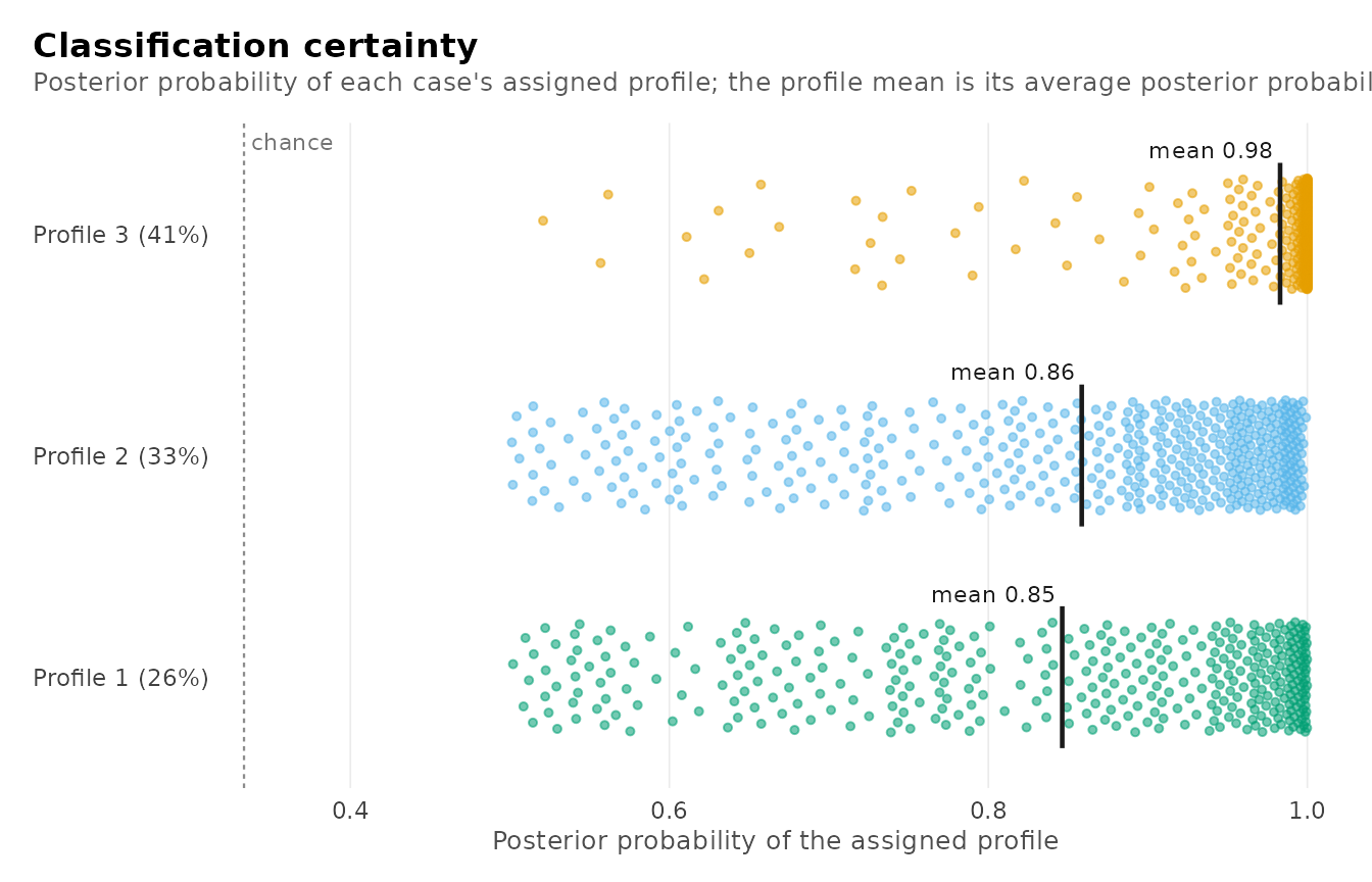

Both levels retain uncertainty, so an analysis that replaces the posteriors by modal assignments treats some enrolments and students as more certain than the model estimates them to be.

Transition networks

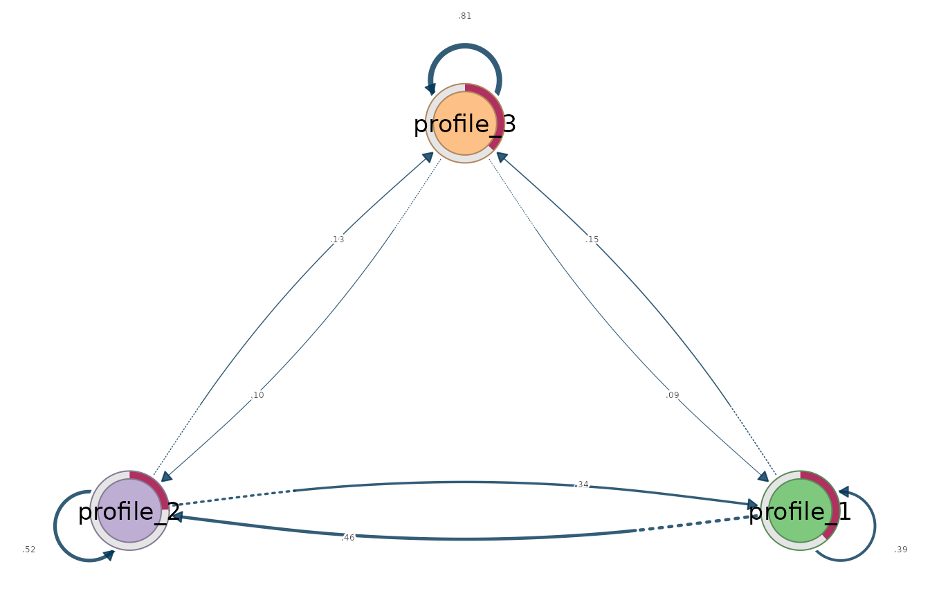
get_tna() returns the marginal transition matrix as a model of the tna package (Tikka et al., 2025). It pools the posterior expected transition counts across classes and normalizes them, so it uses the estimated transitions, not transitions counted from modal assignments. get_group_tna() returns one network per class.

network <- get_tna(moves)
plot(network)

per_class <- get_group_tna(moves)
plot(per_class)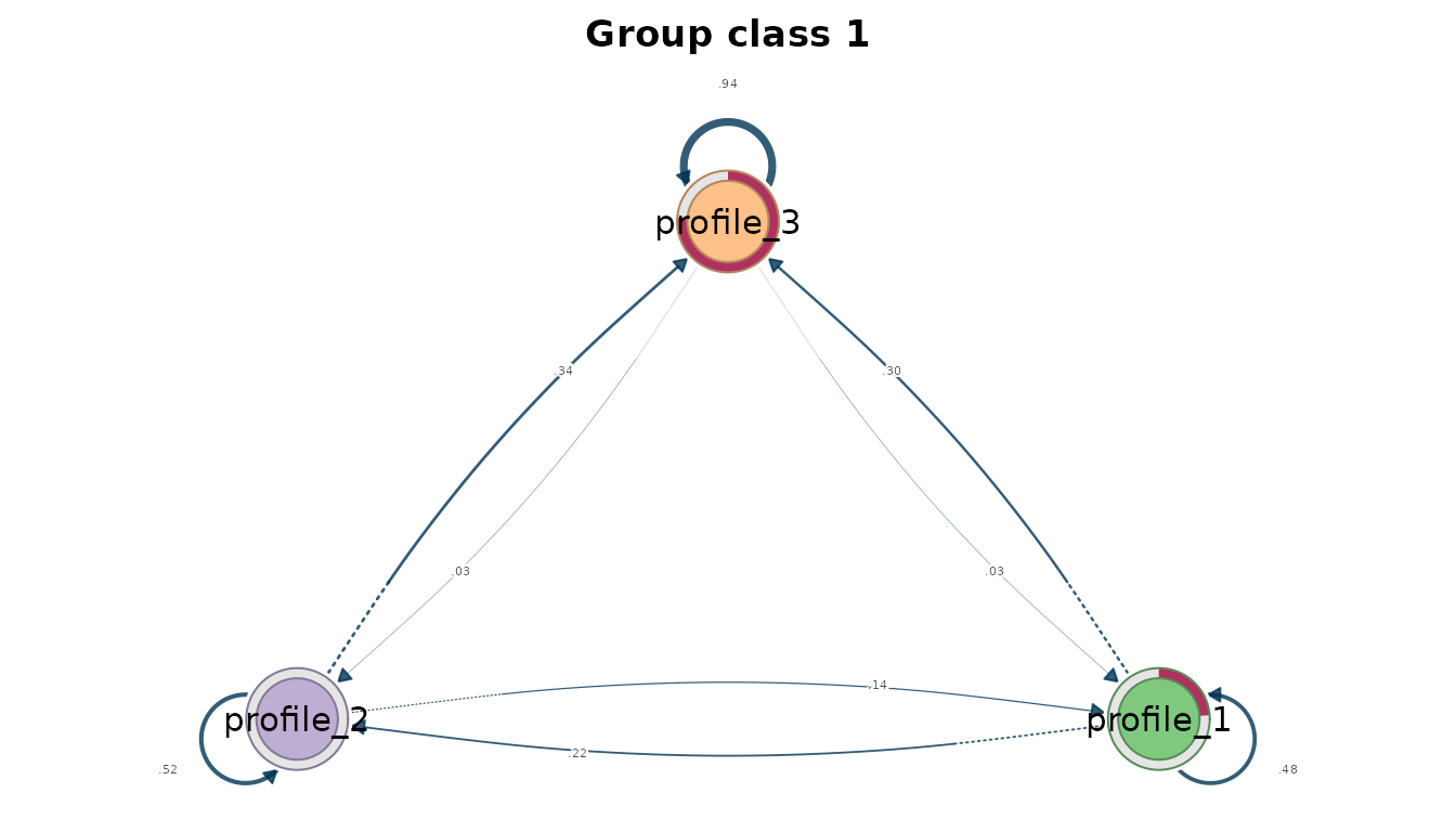

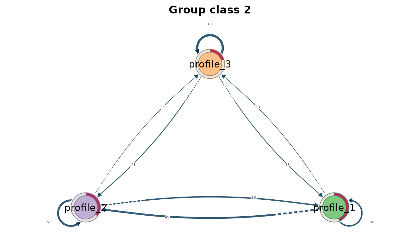
The class networks show the two patterns of the transition table: a dominant self-loop on the lower profile in class 1, and movement among all three profiles in class 2.

Limitations

The model assumes constant transition probabilities across course positions, so change specific to one stage of the program is averaged over positions. Transitions are between successive observed courses, which can differ in duration, content and assessment. Class differences describe patterns in engagement histories and do not identify their causes. Standard errors, likelihood-ratio tests and class enumeration are not available for transition models, so the number of profiles and classes here is a working choice. The diagonal covariance ignores the association between attendance and the click measures, which the evaluation vignette shows is present in these data; unmodelled dependence can be absorbed by extra profiles and change the apparent transitions. Transitions supported by few expected counts, such as those out of the higher and intermediate profiles in class 1, should not be interpreted.

References

Collins, L. M., & Lanza, S. T. (2010). Latent class and latent transition analysis. Wiley.

Saqr, M., & López-Pernas, S. (2021). The longitudinal trajectories of online engagement over a full program. Computers & Education, 175, 104325. https://doi.org/10.1016/j.compedu.2021.104325

Tikka, S., López-Pernas, S., & Saqr, M. (2025). tna: An R package for transition network analysis. Applied Psychological Measurement. https://doi.org/10.1177/01466216251348840

Written by Mohammed Saqr and Sonsoles López-Pernas