Subgroup-Specific Models with fit_subgroups()

Analytic question

fit_subgroups() fits one model per discovered or supplied subgroup and can compare those models with pooled and individual alternatives. The function takes a panel, outcome, predictors, person identifier, subgroup mapping, and model family. It returns an idiographic_fit with the usual tidy accessors.

fit_subgroups() defaults to scope = "all". The pooled scope estimates one coefficient vector. The subgroup scope estimates one vector per group. The individual scope estimates one vector per person. All scopes predict the same ordered test rows.

Estimate subgroup assignments

find_subgroups() supplies a two-group effect-clustering result. This first stage defines the subgroup mapping used by the fitted models.

subgroup_result <- find_subgroups(analysis_data, y = "effort", x = c("efficacy", "monitoring"), id = "name", method = "effect_clustering", k = 2, reps = 20, time = "day")
groups(subgroup_result, sort_by = "subgroup")
#>    subject subgroup            method stability n_assignments
#> 1   Astrid       g1 effect_clustering 0.9833333            20
#> 2    Diana       g1 effect_clustering 0.9500000            20
#> 3   Fatima       g1 effect_clustering 0.9833333            20
#> 4    Frank       g1 effect_clustering 0.9833333            20
#> 5    Aisha       g2 effect_clustering 0.5428571            20
#> 6    Alice       g2 effect_clustering 0.8285714            20
#> 7    Anika       g2 effect_clustering 0.8285714            20
#> 8    Bjorn       g2 effect_clustering 0.8285714            20
#> 9      Bob       g2 effect_clustering 0.8285714            20
#> 10 Charlie       g2 effect_clustering 0.4571429            20
#> 11    Erik       g2 effect_clustering 0.8285714            20
#> 12     Eve       g2 effect_clustering 0.8000000            20

groups() reports assignments and their resampling stability in Table 1. These labels are estimated quantities. Prediction comparisons should retain that first-stage uncertainty in their interpretation.

Fit and compare three scopes

fit_subgroups() fits linear models for all three scopes. Table 2 reports aggregate held-out metrics.

subgroup_fit <- fit_subgroups(analysis_data, y = "effort", x = c("efficacy", "monitoring"), id = "name", subgroup = subgroup_result, method = "lm", time = "day")
metrics(subgroup_fit, overall = TRUE)
#>        scope model estimator  subject subgroup   n     rmse      mae      bias
#> 1     pooled    lm    native .overall     .all 384 23.22627 18.97802 0.4108068
#> 2   subgroup    lm    native .overall     .all 384 22.77474 18.75270 0.4693698
#> 3 individual    lm    native .overall     .all 384 19.83725 15.68630 0.5814738
#>   r_squared
#> 1 0.2897850
#> 2 0.3171306
#> 3 0.4819235

fit_subgroups() gives the subgroup models an RMSE of about 22.8 in Table 2. The pooled RMSE is about 23.2, and the individual RMSE is about 19.8. The two-group model improves modestly over pooling but does not match the individual models on this split.

Plot the scope comparison

plot_metrics() displays the common held-out metric for pooled, subgroup, and individual scopes. Position and colour distinguish the modelling scopes.

plot_metrics(subgroup_fit, metric = "rmse")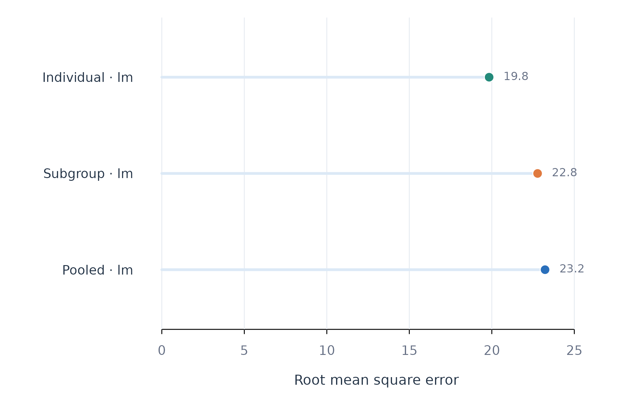

Figure 1. Held-out RMSE for pooled, subgroup, and individual linear models.

Figure 1 shows the subgroup model between the pooled and individual models in prediction error. The result quantifies the compromise between one model for everyone and one model per person.

Assumptions and failure checks

fit_subgroups() treats the supplied mapping as fixed during model fitting. Assignments estimated from the same outcome data can make subgroup performance optimistic. A confirmatory analysis should derive groups in separate data or repeat the complete discovery-and-fitting pipeline within resampling.

fit_subgroups() requires at least one usable training and test set for each requested scope. Small groups can fail even when pooled and individual models succeed. The failure table identifies these cases. Subgroup prediction does not by itself show that discrete populations exist.

When to use which