Rolling-Origin Validation with fit_rolling()

Analytic question

fit_rolling() estimates forecasting performance across several points in time. The function takes a panel, outcome, predictors, person and time columns, a model family, and a rolling schedule. It returns the standard idiographic_fit tables with a fold identifier added to predictions.

fit_rolling() trains on observations before each origin and predicts the next assessment block. The origin then moves forward by step observations. This expanding-window design evaluates a model under repeated historical forecasts instead of one terminal hold-out (Tashman 2000).

Define the rolling schedule

fit_rolling() fits pooled linear models at four origins. Each fold predicts the next five observations per learner. The default initial window uses all earlier rows that can accommodate the requested schedule. Table 1 pools the forecast errors across folds.

rolling_fit <- fit_rolling(analysis_data, y = "effort", x = c("efficacy", "monitoring"), id = "name", method = "lm", time = "day", scope = "pooled", folds = 4, assess = 5)
metrics(rolling_fit, overall = TRUE)
#>    scope model estimator  subject subgroup   n     rmse      mae     bias
#> 1 pooled    lm    native .overall     .all 240 23.78501 19.45259 1.371596
#>   r_squared
#> 1 0.2761391

fit_rolling() evaluates 240 forecasts in Table 1. This count equals four folds, five test occasions, and 12 learners. The pooled linear model has an RMSE of about 23.8 and a positive mean error of about 1.4. These metrics summarize repeated forward predictions rather than in-sample fit.

Inspect fold-level predictions

predictions() returns one row per forecast with the original row identifier, person, observed value, predicted value, and fold. Table 2 limits printing through the accessor’s n argument.

predictions(rolling_fit, n = 12)
#>     scope model estimator subject subgroup row  observed predicted   residual
#> 1  pooled    lm    native   Aisha     .all 137  80.95238  68.45741  12.494971
#> 2  pooled    lm    native   Aisha     .all 138  80.95238  49.32807  31.624313
#> 3  pooled    lm    native   Aisha     .all 139  84.12698  43.85888  40.268099
#> 4  pooled    lm    native   Aisha     .all 140  28.57143  57.50990 -28.938475
#> 5  pooled    lm    native   Aisha     .all 141  90.47619  64.34455  26.131636
#> 6  pooled    lm    native   Alice     .all 293  62.16216  38.52866  23.633499
#> 7  pooled    lm    native   Alice     .all 294  48.64865  52.61346  -3.964814
#> 8  pooled    lm    native   Alice     .all 295  27.02703  41.37232 -14.345294
#> 9  pooled    lm    native   Alice     .all 296  86.48649  59.62317  26.863316
#> 10 pooled    lm    native   Alice     .all 297 100.00000  42.74647  57.253525
#> 11 pooled    lm    native   Anika     .all 449  18.98734  36.55862 -17.571282
#> 12 pooled    lm    native   Anika     .all 450  92.40506  75.07980  17.325262
#>    fold
#> 1     1
#> 2     1
#> 3     1
#> 4     1
#> 5     1
#> 6     1
#> 7     1
#> 8     1
#> 9     1
#> 10    1
#> 11    1
#> 12    1

predictions() shows that each row belongs to a specific forecast origin in Table 2. The fold column permits error review by historical period without reaching into the fitted object.

Plot forecast trajectories

plot_predictions() draws observed and predicted values in row order for selected learners. Figure 1 uses three learner panels.

plot_predictions(rolling_fit, scope = "pooled", n_subjects = 3)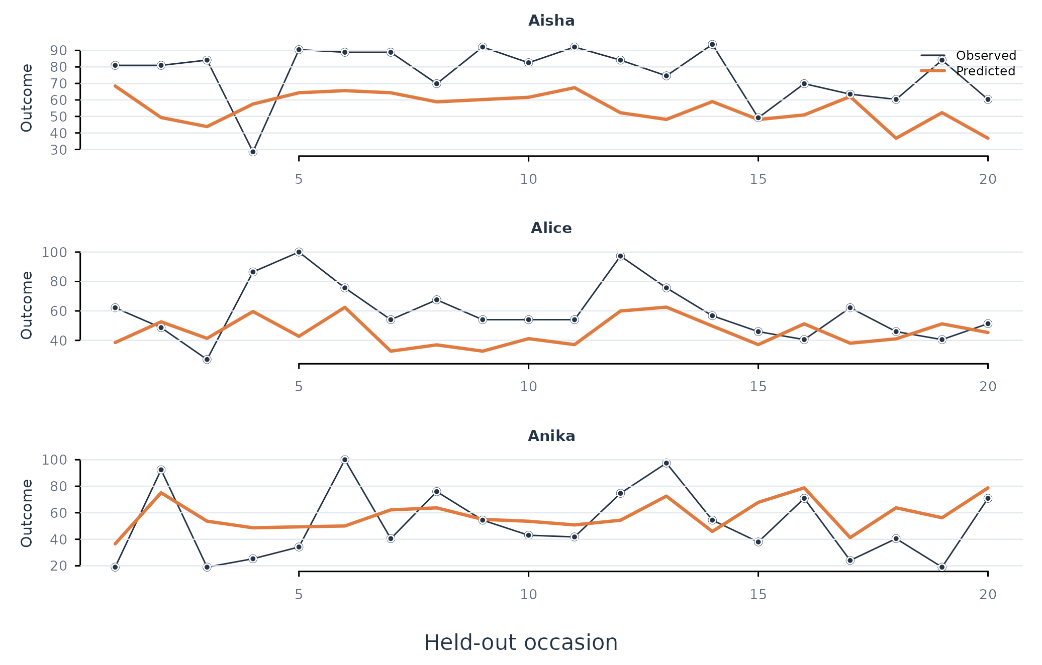

Figure 1. Observed effort and pooled rolling-origin predictions for three learners.

Figure 1 shows where the pooled forecast follows or misses each learner’s held-out trajectory. The plot retains person labels even though one coefficient vector is fitted at the pooled scope.

Assumptions and failure checks

fit_rolling() requires ordered observations and a schedule that fits the shortest person series. The function stops when initial, assess, step, and folds require more rows than are available. Missing predictor or outcome values can reduce usable rows within a fold.

fit_rolling() can tune machine-learning models inside each fold. Validation rows are taken from that fold’s training period. The assessment block remains unseen during tuning. Overlapping assessment blocks occur when step is smaller than assess; metrics then count some time regions more than once.

When to use which

fit_rolling() is appropriate for repeated prospective evaluation. fit_lm(), fit_glm(), and fit_ml() use one terminal hold-out and are appropriate for a single train-test comparison. Rolling network functions address time-varying multivariate systems and have a different result contract.

References

Tashman, Leonard J. 2000. “Out-of-Sample Tests of Forecasting Accuracy: An Analysis and Review.” International Journal of Forecasting 16 (4): 437–50. https://doi.org/10.1016/S0169-2070(00)00065-0.