Stabilizing Person-Specific Coefficients with shrink

Analytic question

shrink_coefs() stabilizes each person’s coefficient using the pooled coefficient distribution. The function takes a fit with individual estimates and standard errors. It returns one tidy row per person and term with the raw estimate, standard error, shrinkage weight, and shrunken estimate.

shrink_coefs() uses an empirical-Bayes rule. The shrinkage weight is the estimated between-person variance divided by that variance plus the person’s sampling variance. A weight near one retains most of the person’s raw estimate. A weight near zero moves the estimate toward the pooled mean.

Estimate individual slopes

fit_lm() estimates separate effort regressions for the 12 learners. The efficacy term is retained because its person-specific slopes and standard errors are the quantities of interest.

individual_fit <- fit_lm(analysis_data, y = "effort", x = c("efficacy", "monitoring"), id = "name", time = "day", scope = "individual")
coefs(individual_fit, scope = "individual", n = 8)
#>        scope model estimator subject subgroup        term   estimate  std_error
#> 1 individual    lm    native   Aisha    .none (Intercept) 60.8053781 4.48242570
#> 2 individual    lm    native   Aisha    .none    efficacy  0.2209651 0.08212755
#> 3 individual    lm    native   Aisha    .none  monitoring  0.1495086 0.06851997
#> 4 individual    lm    native   Alice    .none (Intercept) 64.5515532 6.45537709
#> 5 individual    lm    native   Alice    .none    efficacy  0.4543041 0.07660304
#> 6 individual    lm    native   Alice    .none  monitoring -0.3276520 0.08001883
#> 7 individual    lm    native   Anika    .none (Intercept) 23.1867445 5.98939755
#> 8 individual    lm    native   Anika    .none    efficacy  0.4923880 0.10132704
#>   statistic      p_value
#> 1 13.565284 4.720708e-26
#> 2  2.690512 8.143071e-03
#> 3  2.181971 3.104404e-02
#> 4  9.999656 1.589570e-17
#> 5  5.930628 2.933652e-08
#> 6 -4.094686 7.669590e-05
#> 7  3.871298 1.760110e-04
#> 8  4.859394 3.568461e-06

coefs() displays raw person-specific estimates in Table 1. Differences among these values contain both process heterogeneity and sampling error. Ranking learners by the raw values would treat both sources as substantive.

Apply empirical-Bayes shrinkage

shrink_coefs() estimates the pooled distribution and applies a learner-specific weight. Table 2 retains only the efficacy term through a public argument.

shrunken_coefs <- shrink_coefs(individual_fit, term = "efficacy")
shrunken_coefs
#> SHRUNKEN PERSON EFFECTS
#>   People   12
#>   Terms    1
#> 
#>   subject   term           raw     S.E.   weight   shrunken
#> -----------------------------------------------------------
#>   Aisha     efficacy    0.2210   0.0821    0.852     0.2307
#>   Alice     efficacy    0.4543   0.0766    0.868     0.4322
#>   Anika     efficacy    0.4924   0.1013    0.790     0.4493
#>   Astrid    efficacy   -0.0540   0.0988    0.799     0.0146
#>   Bjorn     efficacy    0.3237   0.0778    0.865     0.3187
#>   Bob       efficacy    0.5820   0.0878    0.834     0.5330
#>   Charlie   efficacy    0.3627   0.1169    0.739     0.3428
#>   Diana     efficacy   -0.0288   0.1282    0.702     0.0652
#>   Erik      efficacy    0.5462   0.1138    0.749     0.4811
#>   Eve       efficacy    0.3975   0.0689    0.891     0.3854
#>   Fatima    efficacy   -0.0745   0.1075    0.770     0.0085
#>   Frank     efficacy    0.1166   0.1487    0.636     0.1785
#> 
#>   weight = how much of the person's own estimate is kept

shrink_coefs() moves every efficacy slope toward the pooled efficacy effect in Table 2. Learners with larger standard errors receive smaller weights and move farther. The shrunken values preserve estimated heterogeneity while reducing the influence of measurement noise.

Plot raw and shrunken estimates

The paired-dot display places learners on rows and coefficients on the horizontal axis. Each line begins at the raw estimate and ends at the shrunken estimate, making both the direction and size of shrinkage visible.

shrunken_coefs <- shrunken_coefs[order(shrunken_coefs$shrunken), ]
at <- seq_len(nrow(shrunken_coefs))
limits <- range(c(shrunken_coefs$estimate, shrunken_coefs$shrunken, 0))
figure_begin(c(4.2, 7, 1, 1))
plot(shrunken_coefs$shrunken, at, xlim = limits,
     ylim = c(0.5, length(at) + 0.5), yaxt = "n", pch = 21,
     bg = fig_col["teal"], col = "white", cex = 1.3,
     xlab = "Efficacy coefficient", ylab = "")
figure_grid(x = TRUE, y = FALSE)
abline(v = 0, col = fig_col["muted"], lty = 2)
segments(shrunken_coefs$estimate, at, shrunken_coefs$shrunken, at,
         col = fig_col["grid"], lwd = 2.4)
points(shrunken_coefs$estimate, at, pch = 21, bg = "white",
       col = fig_col["muted"], cex = 1.05)
points(shrunken_coefs$shrunken, at, pch = 21, bg = fig_col["teal"],
       col = "white", cex = 1.3)
axis(2, at = at, labels = shrunken_coefs$subject, tick = FALSE,
     col.axis = fig_col["ink"])
legend("bottomright", c("Raw", "Shrunken"), pch = 21,
       pt.bg = c("white", fig_col["teal"]),
       col = c(fig_col["muted"], "white"), bty = "n", cex = 0.8)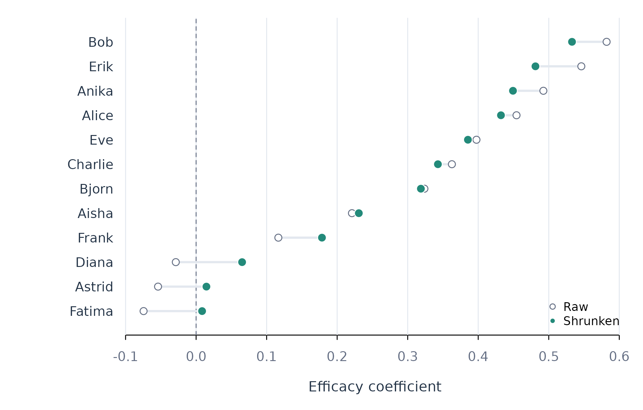

Figure 1. Raw and empirical-Bayes efficacy coefficients for 12 learners.

Figure 1 shows the raw-to-shrunken movement explicitly. Extreme raw values move towards the pooled centre, while precise estimates move less. The plot should be interpreted with the weight column in Table 2: longer connecting lines indicate that the individual’s estimate carried less weight.

Assumptions and failure checks

shrink_coefs() inherits the random-effects assumptions of pool_coefs(). The method assumes independent people and a coefficient distribution that can be summarized by one mean and variance. A multimodal coefficient distribution can make one pooled centre inadequate.

shrink_coefs() requires standard errors. It does not accept coefficient tables that assign equal certainty without evidence. Shrinkage estimates are appropriate for description and stabilized prediction. Their usual intervals require additional modelling if formal person-specific inference is the goal.

When to use which

shrink_coefs() is appropriate for stabilized person-level estimates. pool_coefs() is appropriate for the population mean and between-person spread. test_subgroups() is appropriate before replacing one coefficient distribution with discrete classes. Raw individual coefficients remain useful when each person has enough information and minimal sampling error.