Pooled and Person-Specific Linear Models with fit

Analytic question

fit_lm() estimates a continuous outcome from one or more predictors at pooled, subgroup, or person-specific scopes. The function takes a long-format panel and column names for the outcome, predictors, person, and optional time order. It returns an idiographic_fit with tidy coefficients, held-out predictions, performance metrics, and failures.

fit_lm() uses an ordered hold-out within each learner. Earlier observations form the training set and the final proportion forms the test set. The pooled model shares one coefficient vector across learners. The individual scope fits one coefficient vector per learner.

Fit both scopes

fit_lm() models daily effort from efficacy and monitoring. The default scope = "both" fits pooled and individual models using the same ordered test rows. Table 1 compares their aggregate held-out performance.

lm_fit <- fit_lm(analysis_data, y = "effort", x = c("efficacy", "monitoring"), id = "name", time = "day", scope = "both")
metrics(lm_fit, overall = TRUE)
#>        scope model estimator  subject subgroup   n     rmse      mae      bias
#> 1     pooled    lm    native .overall     .all 384 23.22627 18.97802 0.4108068
#> 2 individual    lm    native .overall     .all 384 19.83725 15.68630 0.5814738
#>   r_squared
#> 1 0.2897850
#> 2 0.4819235

fit_lm() gives the individual models a lower RMSE than the pooled model in Table 1. The individual aggregate RMSE is about 19.8, compared with 23.2 for the pooled model. The corresponding held-out R-squared values are about 0.48 and 0.29. These figures describe this panel and this split.

Inspect person-specific coefficients

coefs() retrieves inferential estimates without accessing the fit’s internal list. Table 2 reports Aisha’s individual regression.

coefs(lm_fit, scope = "individual", subject = "Aisha")
#>        scope model estimator subject subgroup        term   estimate  std_error
#> 1 individual    lm    native   Aisha    .none (Intercept) 60.8053781 4.48242570
#> 2 individual    lm    native   Aisha    .none    efficacy  0.2209651 0.08212755
#> 3 individual    lm    native   Aisha    .none  monitoring  0.1495086 0.06851997
#>   statistic      p_value
#> 1 13.565284 4.720708e-26
#> 2  2.690512 8.143071e-03
#> 3  2.181971 3.104404e-02

coefs() reports positive efficacy and monitoring coefficients for Aisha in Table 2. Each coefficient is conditional on the other predictor. The standard errors and p-values describe uncertainty in the training-period regression. They do not measure held-out prediction error.

Plot held-out predictions

plot_predictions() compares observed and predicted test values for selected learners. Figure 1 displays three individual models. Black points and lines are observations. Orange lines are predictions.

plot_predictions(lm_fit, scope = "individual", n_subjects = 3)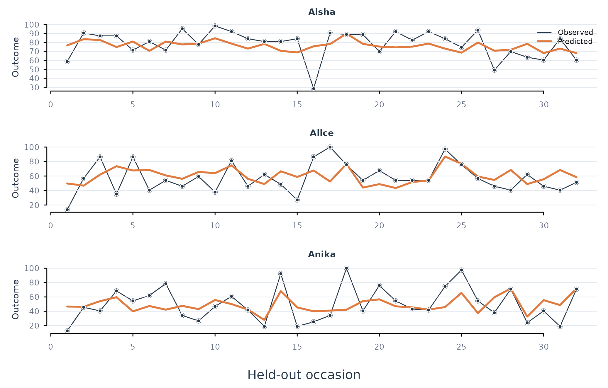

Figure 1. Held-out effort and person-specific linear-model predictions for three learners.

Figure 1 shows that prediction quality differs across learners and occasions. The aggregate advantage in Table 1 does not imply equal accuracy for every person. The trajectory plot should accompany aggregate metrics when the unit of inference is the person.

Assumptions and failure checks

fit_lm() assumes a linear conditional mean, finite residual variance, and a training period that represents the test period. Coefficient intervals also use the fitted linear-model sampling assumptions. Serially correlated residuals can make those intervals too narrow. Held-out metrics remain useful for prediction even when coefficient inference requires a richer error model.

fit_lm() records persons with insufficient complete training or test rows in the failure table. The function does not move observations across person boundaries to fill a split. The optional weights argument names a case-weight column. The estimator = "robust" option uses MASS::rlm() when resistance to outlying residuals is required.

When to use which

fit_lm() is appropriate for a continuous outcome and interpretable linear coefficients. fit_glm() is appropriate for binary, count, and other supported response families. fit_ml() is appropriate when held-out prediction and nonlinear algorithms are primary. fit_within_between() is appropriate when raw predictors would mix within-person and between-person effects.