Repeated-Split Heterogeneity Analysis with fit_heterogeneity() • idiographic

Analytic question

fit_heterogeneity() tests whether a person-varying quantity differs systematically across people. The target can be a treatment effect, prediction error, or gain from individual rather than pooled modelling. The function returns repeated-split estimates, sorted groups, a heterogeneity slope, characteristics of extreme groups, and learner-selection criteria.

fit_heterogeneity() separates proxy learning from inference. One sample learns a machine-learning proxy for the person-varying target. A held-out sample estimates average, grouped, and heterogeneity quantities. Repeating and aggregating the split reduces dependence on one random partition (Chernozhukov et al. 2020). Standard errors cluster observations by person.

Study heterogeneity in prediction error

fit_heterogeneity() asks whether effort prediction error varies predictably across learners. Linear and ridge proxies compete over ten person-level random splits. Three sorted groups range from lower to higher error.

heterogeneity_fit <- fit_heterogeneity(analysis_data, y = "effort", x = c("efficacy", "monitoring", "planning"), id = "name", target = "error", model = c("linear", "ridge"), num_splits = 10, n_groups = 3)
heterogeneity(heterogeneity_fit)
#>   target model           effect   estimate std_error   conf_low conf_high
#> 1  error ridge          average 20.2253550 1.7855913 15.2771405  24.96474
#> 2  error ridge    heterogeneity  0.6435549 0.5969202 -0.8915956   1.88939
#> 3  error ridge         group:g1 19.9370663 2.1115599 15.0984244  24.79795
#> 4  error ridge         group:g2 19.9644428 2.0247641 14.7204603  25.09312
#> 5  error ridge         group:g3 21.9773560 2.8928578 14.6957330  28.46461
#> 6  error ridge group:top-bottom  2.9556581 3.0949341 -6.4277446  10.72051
#>        p_value   n n_people splits
#> 1 0.0001857984 933        6     10
#> 2 0.5792993199 933        6     10
#> 3 0.0004026063 933        6     10
#> 4 0.0003792906 933        6     10
#> 5 0.0012330464 933        6     10
#> 6 0.8202282399 933        6     10

heterogeneity() reports an average absolute prediction error of about 20.2 in Table 1. The highest-minus-lowest group contrast is about 3.0, and its interval includes zero. The heterogeneity slope interval also includes zero. The analysis does not find stable, predictable error heterogeneity in this 12-learner subset.

Describe and compare learned proxies

clan() compares predictor means between extreme target groups. learners() reports the criterion used to select the proxy model.

clan(heterogeneity_fit)
#>   target model   variable  estimate std_error  conf_low  conf_high      p_value
#> 1  error ridge   efficacy -25.86529  8.736283 -42.19034  -5.789263 0.1280360561
#> 2  error ridge monitoring -52.86498  5.479528 -63.46382 -42.450660 0.0004350839
#> 3  error ridge   planning -30.30356  5.186209 -39.11614 -30.308775 0.0084234023
#>     n n_people splits
#> 1 622        6     10
#> 2 622        6     10
#> 3 622        6     10
learners(heterogeneity_fit)
#>    model   lambda lambda_bar
#> 1  ridge 2.167416   409.5028
#> 2 linear 2.152740   409.5413

clan() reports descriptive differences between extreme predicted-error groups in Table 2. These differences describe the fitted grouping and do not identify causes of prediction error. learners() selects ridge by a small criterion difference in Table 3.

Plot the heterogeneity estimates

The coefficient-and-interval display includes the average, heterogeneity slope, sorted groups, and extreme-group contrast. Unlike a point-only plot, it keeps the uncertainty required for the substantive conclusion.

heterogeneity_table <- heterogeneity(heterogeneity_fit)
heterogeneity_labels <- c(
  average = "Average absolute error",
  heterogeneity = "Heterogeneity slope",
  `group:g1` = "Lowest-error group",
  `group:g2` = "Middle-error group",
  `group:g3` = "Highest-error group",
  `group:top-bottom` = "Highest minus lowest"
)
labels <- unname(heterogeneity_labels[heterogeneity_table$effect])
forest_plot(heterogeneity_table$estimate, heterogeneity_table$conf_low,
            heterogeneity_table$conf_high, labels,
            xlab = "Absolute-error target (95% CI)", colour = fig_col["purple"])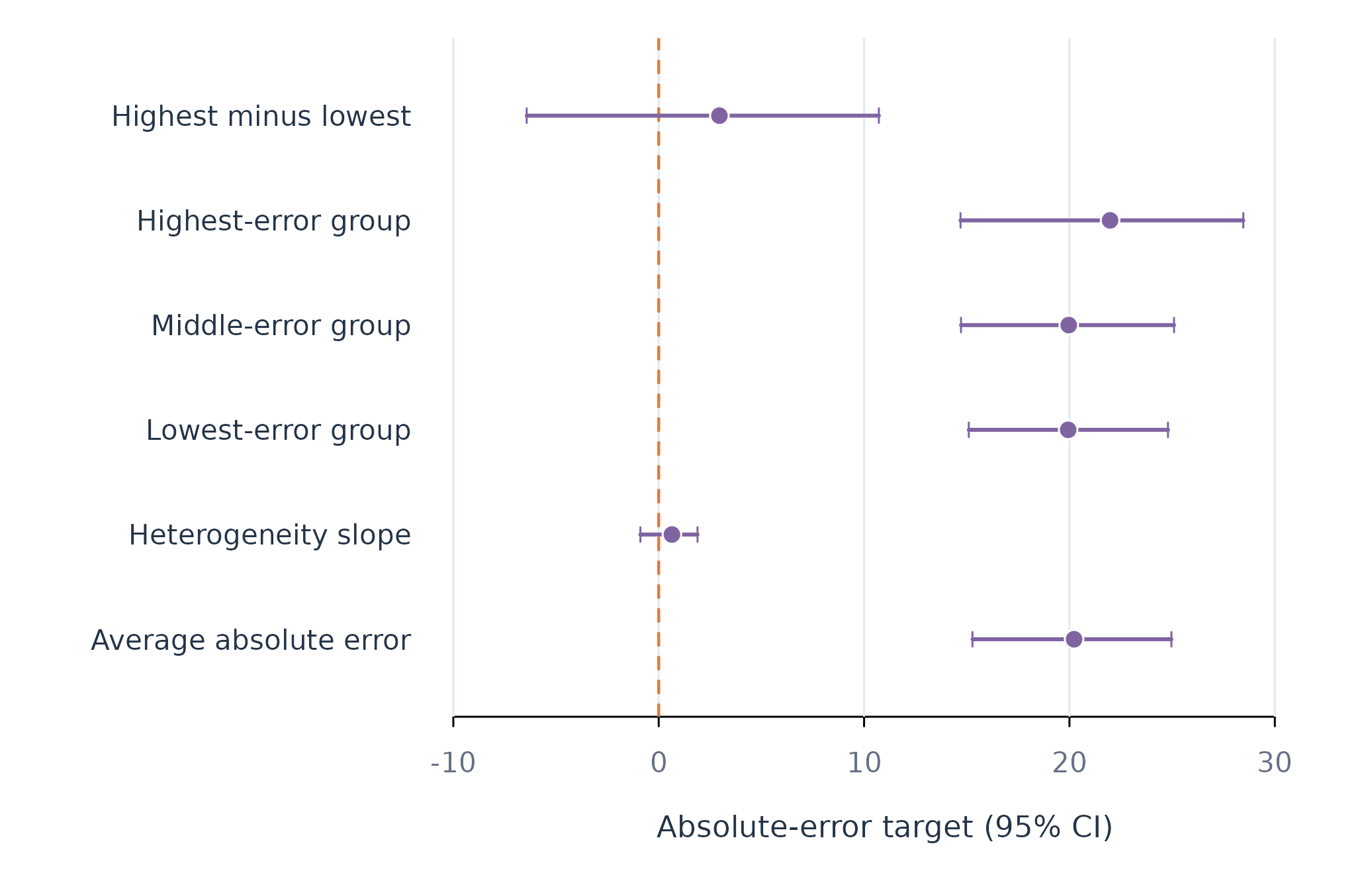

Figure 1. Repeated-split estimates for average error and error heterogeneity.

Figure 1 shows similar estimates for the three error groups and wide uncertainty for their contrast. The heterogeneity-slope and highest-minus-lowest intervals cross zero, so this analysis does not establish systematic error heterogeneity.

Assumptions and failure checks

fit_heterogeneity() treats people as independent clusters for the default person split. The number of independent people limits precision even when each person contributes many rows. More random splits reduce split sensitivity but do not create additional independent units.

fit_heterogeneity() uses random rather than time-ordered splits because its target is cross-person heterogeneity. The gain target changes to occasion splits so each person appears in both modelling samples. Forecast evaluation should use fit_rolling() instead. A causal interpretation of the cate target requires the same identification assumptions as fit_effects().

When to use which

fit_heterogeneity() is appropriate for repeated-split inference about a person-varying target. fit_effects() is appropriate for direct average and sorted treatment-effect estimation across model scopes. test_subgroups() is appropriate when the question concerns discrete coefficient populations. fit_rolling() is appropriate for change in prediction performance over time.

References

Chernozhukov, Victor, Mert Demirer, Esther Duflo, and Ivan Fernandez-Val. 2020. “Generic Machine Learning Inference on Heterogeneous Treatment Effects in Randomized Experiments.” arXiv. https://arxiv.org/abs/1712.04802.