Person-Level Description with describe_persons() • idiographic

Analytic question

describe_persons() answers whether each person’s repeated series contains enough variation, temporal coverage, and usable observations for an idiographic analysis. The function takes a long-format panel, variable names, a person identifier, and an optional ordering variable. It returns one tidy row per person and variable.

describe_persons() separates overall dispersion from successive change. The standard deviation measures dispersion around a person’s mean. The root mean square successive difference measures movement between adjacent occasions. These quantities describe different temporal patterns (Jahng et al. 2008). The lag-one autocorrelation measures carry-over from one occasion to the next.

Estimate person-level summaries

describe_persons() uses time = "day" to order observations within each learner. The detail = "full" setting adds floor and ceiling proportions, acute-change probability, skewness, kurtosis, linear trend, and the longest run of repeated values. Table 1 reports two learners and two variables so the full output remains readable.

descriptives <- describe_persons(analysis_data, id = "name", vars = c("efficacy", "effort"), time = "day", subject = c("Aisha", "Alice"), detail = "full")
descriptives
#> PERSON DESCRIPTIVES
#>   Grouping    name
#>   Time        day
#>   People      2
#>   Variables   2
#> 
#>   subject   variable     n   miss     mean   median       sd     min       max    rmssd   autocor      span   gap_median   gap_max   p_floor   p_ceiling     pac     skew   kurtosis    trend   trend_p   longest_run
#> ---------------------------------------------------------------------------------------------------------------------------------------------------------------------------------------------------------------------
#>   Aisha     efficacy   156      0   56.919   61.765   21.034   0.000   100.000   26.881     0.169   155.000        1.000     1.000     0.006       0.019   0.071   -0.669      0.285    0.054     0.152         2.000
#>   Alice     efficacy   156      0   35.761   36.364   20.614   0.000   100.000   28.790     0.024   155.000        1.000     1.000     0.026       0.013   0.065    0.395     -0.193   -0.013     0.734         2.000
#>   Aisha     effort     156      0   77.646   82.540   18.080   0.000   100.000   23.724     0.132   155.000        1.000     1.000     0.019       0.026   0.039   -2.020      5.489    0.008     0.793         2.000
#>   Alice     effort     156      0   59.875   60.811   21.108   0.000   100.000   30.319    -0.032   155.000        1.000     1.000     0.019       0.019   0.071   -0.468      0.084    0.025     0.512         3.000
#> 
#>   sd    = overall spread;  rmssd = occasion-to-occasion change
#>   autocor = lag-1 carry-over (inertia)

describe_persons() reports 156 observations for each displayed series in Table 1. Aisha’s efficacy mean is higher than Alice’s, while their efficacy RMSSD values are similar. The result therefore distinguishes a difference in typical level from a difference in occasion-to-occasion movement. The gap columns equal one day for these learners, so a lag represents a consistent elapsed interval.

Plot dispersion against successive change

The figure compares standard deviation with RMSSD and labels every series directly. Position, colour, and symbol jointly identify the variable and learner; the labels make the figure interpretable without a separate lookup.

point_col <- ifelse(descriptives$variable == "efficacy", fig_col["blue"], fig_col["orange"])
point_pch <- ifelse(descriptives$subject == "Aisha", 21, 24)
labels <- paste(descriptives$subject, descriptives$variable, sep = " · ")
figure_begin(c(4.2, 4.8, 1, 2.2))
plot(descriptives$sd, descriptives$rmssd,
     xlim = range(descriptives$sd) + c(-1, 1) * diff(range(descriptives$sd)) * 0.12,
     ylim = range(descriptives$rmssd) + c(-1, 1) * diff(range(descriptives$rmssd)) * 0.12,
     pch = point_pch, bg = point_col, col = "white", cex = 1.5,
     xlab = "Person-level standard deviation",
     ylab = "Root mean square successive difference")
figure_grid(x = TRUE, y = TRUE)
points(descriptives$sd, descriptives$rmssd, pch = point_pch,
       bg = point_col, col = "white", cex = 1.5)
text(descriptives$sd, descriptives$rmssd, labels = labels, pos = 4,
     offset = 0.65, cex = 0.76, col = fig_col["ink"], xpd = TRUE)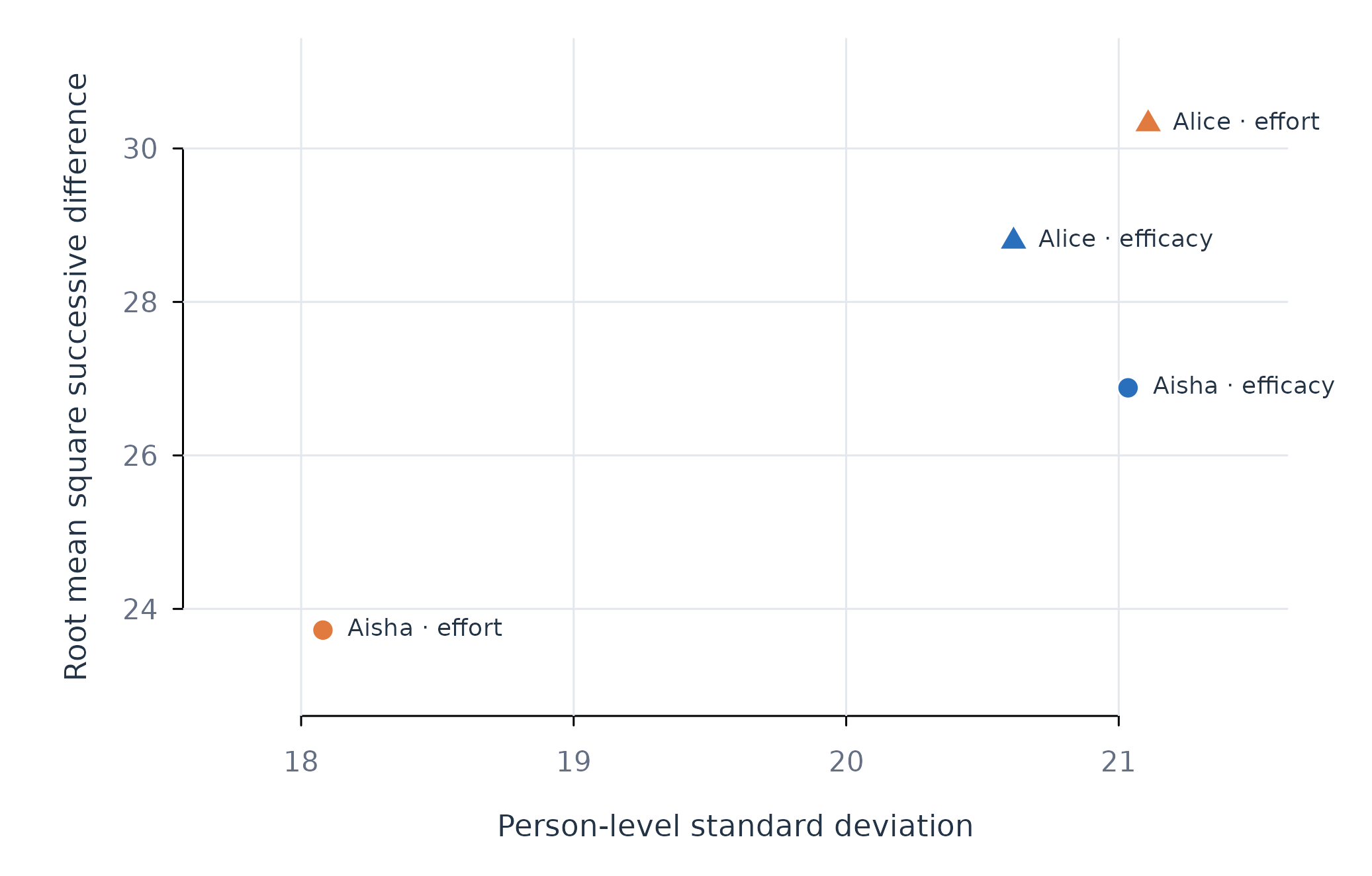

Figure 1. Overall dispersion and successive change for efficacy and effort in two learners.

Figure 1 shows that overall spread and short-term movement do not occupy one common scale. A series can vary widely across the observation period without changing by the same amount between adjacent days. Both quantities should be reported when temporal instability is substantively relevant.

Assumptions and failure checks

describe_persons() treats successive rows as adjacent only after ordering within person. The time argument is therefore required when row order is not the intended chronology. Missing values reduce the usable pair count for RMSSD and autocorrelation. A constant series has no estimable correlation and cannot support a person-specific slope.

describe_persons() defines acute change relative to the pooled sample unless pac_cutoff is supplied. Analyses that compare acute-change rates across datasets should use a common substantive cutoff. The trend and trend_p columns describe a linear trend. They do not diagnose every form of nonstationarity.

When to use which

describe_persons() is the first choice for person-level data sufficiency, location, variability, movement, and timing. correlate_persons() addresses pairwise within-person association. variance_components() quantifies how much sample variance lies within and between people. Model-fitting functions should follow these checks when the available variation supports the intended estimand.

References

Jahng, Seungmin, Phillip K. Wood, and Timothy J. Trull. 2008. “Analysis of Affective Instability in Ecological Momentary Assessment: Indices Using Successive Difference and Group Comparison via Multilevel Modeling.” Psychological Methods 13 (4): 354–75. https://doi.org/10.1037/a0014173.