
Markov Stability Analysis
Mohammed Saqr
University of Eastern FinlandSonsoles López-Pernas
University of Eastern FinlandKamila Misiejuk
FernUniversität in Hagen, GermanySource:
vignettes/markov-stability.Rmd
markov-stability.RmdNestimate provides two functions for Markov-chain stability analysis of transition networks:
-
passage_time()– computes the full matrix of mean first passage times (MFPT). Entry M[i, j] is the expected number of steps to travel from state i to state j for the first time. The diagonal equals the mean recurrence time 1/pi. -
markov_stability()– computes per-state stability metrics: persistence, stationary probability, return time, sojourn time, and mean accessibility.
Both functions accept a netobject,
cograph_network, tna object, row-stochastic
matrix, or a raw wide sequence data frame.
Data
trajectories contains 138 learners recorded at 15
time-steps each with three engagement states: Active, Average, and
Disengaged.
dim(trajectories)
#> [1] 138  15
table(as.vector(trajectories), useNA = "always")
#>
#>     Active    Average Disengaged       <NA>
#>        703        813        354        200
Selecting mostly-active learners
Does a learner who is mostly engaged stay out of disengagement for longer, or only visit it less often? To compare, we keep learners who were Active more than half the time (> 7 of 15 steps; missing weeks do not count as Active).
sub <- subset(trajectories, rowSums(trajectories == "Active", na.rm = TRUE) > 7)
nrow(sub)
#> [1] 42

Transition networks
net_all <- build_network(trajectories, method = "relative")
net_sub <- build_network(sub, method = "relative")

net_all
#> Transition Network (relative probabilities) [directed]
#>   Weights: [0.035, 0.698]  |  mean: 0.333
#>
#>   Weight matrix:
#>              Active Average Disengaged
#>   Active      0.698   0.267      0.035
#>   Average     0.204   0.610      0.186
#>   Disengaged  0.120   0.397      0.483
#>
#>   Initial probabilities:
#>   Active        0.382  ████████████████████████████████████████
#>   Average       0.368  ██████████████████████████████████████
#>   Disengaged    0.250  ██████████████████████████
net_sub
#> Transition Network (relative probabilities) [directed]
#>   Weights: [0.017, 0.819]  |  mean: 0.333
#>
#>   Weight matrix:
#>              Active Average Disengaged
#>   Active      0.819   0.164      0.017
#>   Average     0.683   0.288      0.029
#>   Disengaged  0.643   0.143      0.214
#>
#>   Initial probabilities:
#>   Active        0.762  ████████████████████████████████████████
#>   Average       0.238  ████████████
#>   Disengaged    0.000
In the mostly-active group nearly every state transitions predominantly back to Active, and the probability of entering Disengaged is almost zero.
Mean First Passage Times
pt_all <- passage_time(net_all)
pt_sub <- passage_time(net_sub)
print(pt_all, digits = 2)
#> Mean First Passage Times (3 states)
#>
#>            Active Average Disengaged
#> Active       2.69    3.63      10.36
#> Average      5.51    2.26       7.97
#> Disengaged   6.16    2.78       5.41
#>
#> Stationary distribution:
#>     Active    Average Disengaged
#>     0.3719     0.4431     0.1850
print(pt_sub, digits = 2)
#> Mean First Passage Times (3 states)
#>
#>            Active Average Disengaged
#> Active       1.27    6.12      51.99
#> Average      1.47    5.36      51.29
#> Disengaged   1.54    6.28      41.75
#>
#> Stationary distribution:
#>     Active    Average Disengaged
#>     0.7895     0.1866     0.0240
Active to Disengaged rises from 10.4 to 52.0 steps – a mostly-active learner takes five times as long to reach disengagement. The diagonal equals the mean recurrence time (how many steps between consecutive visits to the same state).
plot(pt_all, title = "Full sample (n = 138)")
plot(pt_sub, title = "Mostly-active learners (n = 42)")
In the mostly-active heatmap the Active column is uniformly dark (quickly reachable from any state) and the Disengaged column is uniformly pale (nearly unreachable).
Stationary distribution
The stationary distribution is the long-run share of time spent in
each state. markov_stability() reports it per state as
stationary_prob, beside the other per-state metrics
described in the next section.
ms_all <- markov_stability(net_all)
ms_sub <- markov_stability(net_sub)

summary(ms_all)
#> Most accessible state (attractor): Average
#> Most persistent state (stickiest): Active
#>        state persistence stationary_prob return_time sojourn_time
#> 1     Active      0.6976          0.3719        2.69         3.31
#> 2    Average      0.6099          0.4431        2.26         2.56
#> 3 Disengaged      0.4831          0.1850        5.41         1.93
#>   avg_time_to_others avg_time_from_others
#> 1               6.99                 5.84
#> 2               6.74                 3.20
#> 3               4.47                 9.16
summary(ms_sub)
#> Most accessible state (attractor): Active
#> Most persistent state (stickiest): Active
#>        state persistence stationary_prob return_time sojourn_time
#> 1     Active      0.8191          0.7895        1.27         5.53
#> 2    Average      0.2885          0.1866        5.36         1.41
#> 3 Disengaged      0.2143          0.0240       41.75         1.27
#>   avg_time_to_others avg_time_from_others
#> 1              29.06                 1.50
#> 2              26.38                 6.20
#> 3               3.91                51.64
In the mostly-active group ~79% of long-run time is spent Active (vs 37% in the full sample).
Markov Stability
The per-state table printed above contains:
| Column | Meaning |
|---|---|
persistence |
P[i,i] – probability of staying at the next step |
stationary_prob |
Long-run proportion of time in this state |
return_time |
Expected steps between consecutive visits (1/pi) |
sojourn_time |
Expected consecutive steps before leaving (1/(1-P[i,i])) |
avg_time_to_others |
Mean MFPT leaving this state to all others |
avg_time_from_others |
Mean MFPT from all other states arriving here |
plot(ms_all, title = "Full sample")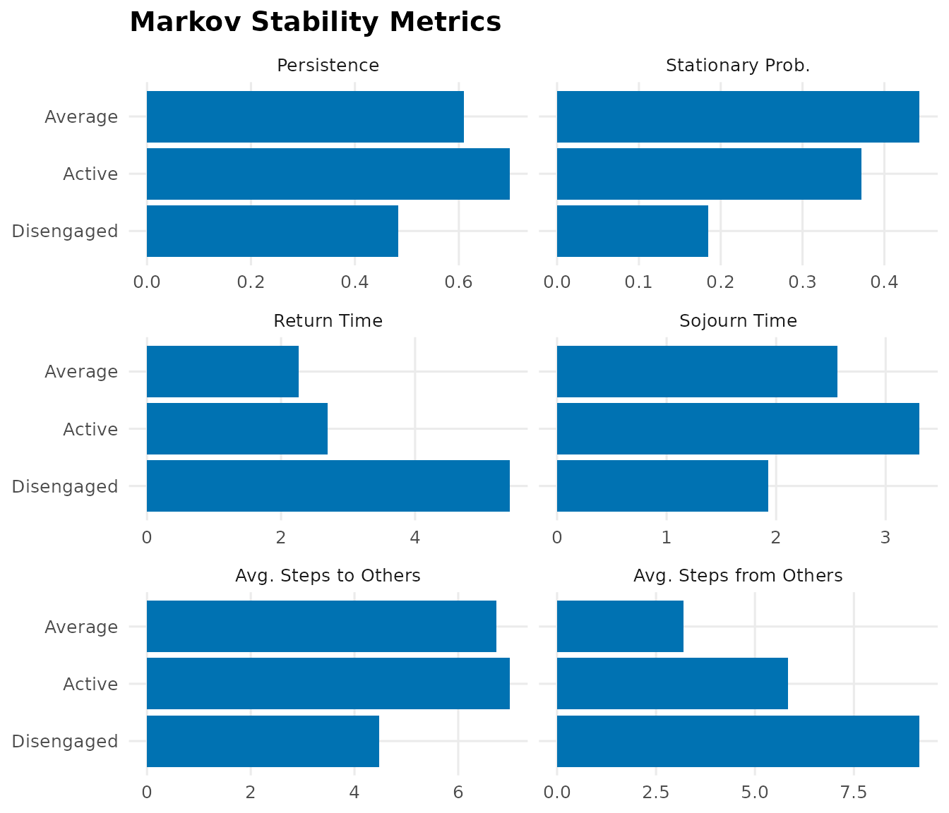
plot(ms_sub, title = "Mostly-active learners")
Among the mostly-active learners, Active leads on persistence (0.82)
and sojourn time (5.5 steps) – once a learner is active they stay active
– and it is also the most accessible state
(avg_time_from_others 1.5 steps). Disengaged has
avg_time_from_others of 51.6 steps – effectively
unreachable. In the full sample the most accessible state is Average
(3.2 steps), and Disengaged is reached in 9.2 steps on average.