Plotting Time Series Networks

Mohammed Saqr

University of Eastern Finland

Sonsoles López-Pernas

University of Eastern Finland

Manuel J. Gómez

University of Murcia

Introduction

Which plot is drawn from a time series network selects which aspect of the data becomes visible: the measured temporal sequence, the states assigned to observations, or the relational structure defined by the network. These views describe different aspects of the same analysis and should not be interpreted as equivalent representations.

The plotting methods in tsn select the representation with the type argument. Additional arguments control the visual encoding within that representation, including state placement, point display, colour, labels, node size, and edge annotation. When type is omitted, plot() uses the default type for the corresponding result class.

This vignette uses one pleasure series throughout. Each analytical object is constructed immediately before its first plot, keeping the relationship between the analysis and its graphical representation explicit.

Result class	Plot types	Default
Discrete states from discretize()	"overlay", "ribbon", "heatmap", "stack"	"overlay"
Local direction from trend()	"points", "ribbon", "heatmap", "panels"	"points"
Network from tsn() or vg()	"network", "series"	"network"
TNA-family model	"combined", "network", "series"	"combined"
Model collection from series_networks()	"network"	"network"

For network objects, "network" displays the nodes and edges defined by the model, whereas "series" shows the source time series from which the network was constructed, with no network structure drawn over it. For TNA-family models, "combined" displays the state sequence together with the corresponding transition network, while "network" focuses on the state-to-state relationships alone. The choice of plot type therefore determines whether the figure is used to examine the temporal sequence, the state representation, or the network structure.

Data

The examples use the first 60 observations of pleasure from the motivation data. A 25-observation segment is used for visibility analysis so that individual nodes and edges remain distinguishable.

data("motivation", package = "tsn")

pleasure <- head(motivation, 60)
short <- head(pleasure, 25)

Discrete-state plots

The plot() method for a tsn_states object provides four representations of the same discretization.

type	Graphical encoding	Scientific use
"overlay"	State value bands behind the measured series	Relating assigned states to their value ranges and boundaries
"ribbon"	State strip beneath an unobscured series	Retaining exact variation when state changes are frequent
"heatmap"	One categorical tile per observation	Displaying the state sequence as a compact temporal signature
"stack"	Companion series aligned above the discretized series	Relating the states of a derived quantity to its source measurement

The principal arguments are type and series. For overlays, overlay selects horizontal ranges (the default), vertical regions, or no shading; lines can add state boundaries; and min_run suppresses very short displayed runs without changing the fitted states. The arguments points, palette, alpha, legend, and grid control graphical appearance. Heatmaps additionally accept sort and border. The stack view requires a numeric companion supplied with with; shade and color_line determine how the state classification is carried across the two panels.

Overlay

The series is first discretized into three empirical quantile states and then plotted. Because "overlay" is the default type, no plotting argument is required.

states <- discretize(
  data = pleasure,
  series = "pleasure",
  labels = c("Low", "Middle", "High")
)

plot(states)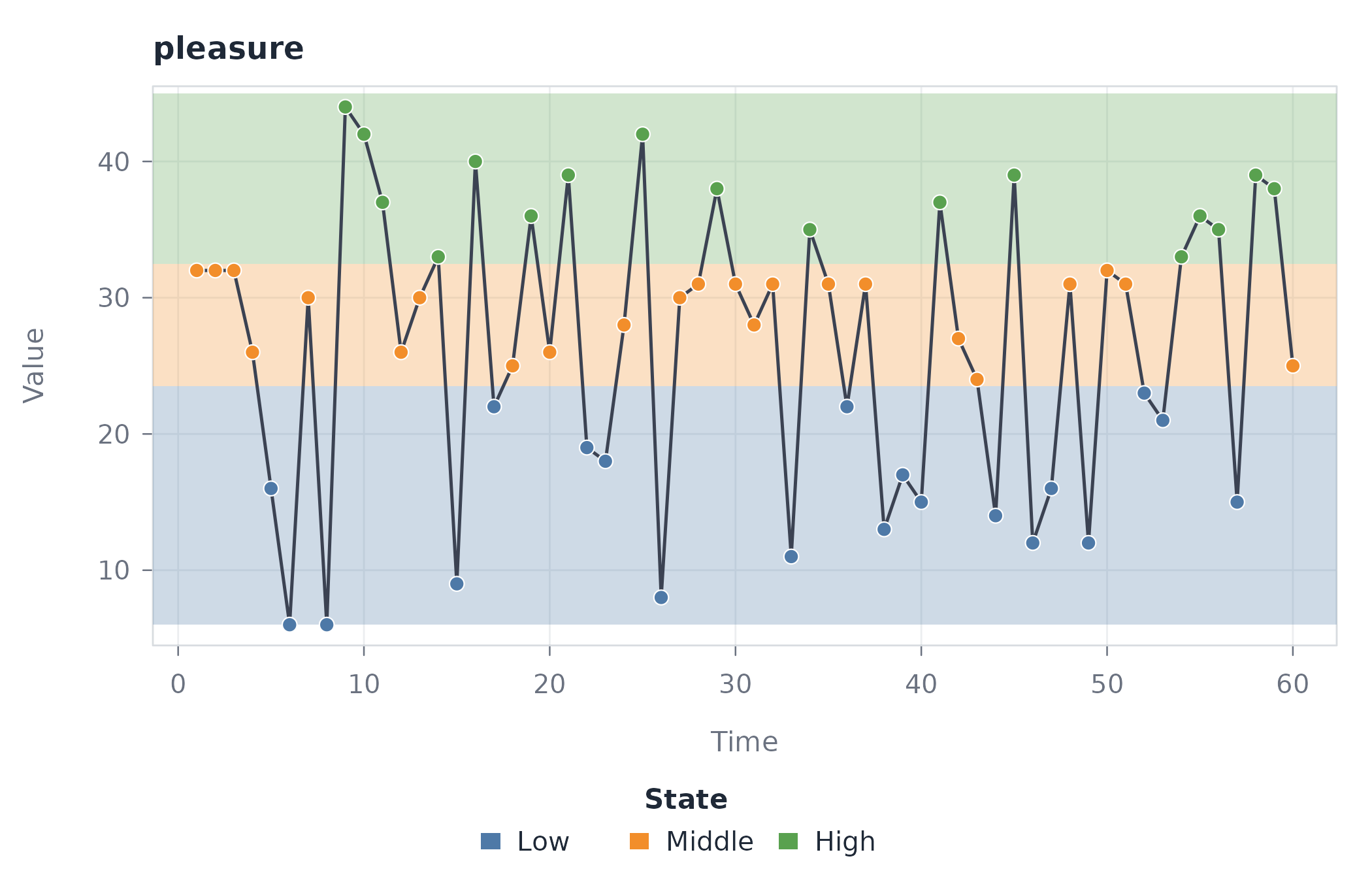

The horizontal bands identify the value ranges associated with the three states, while the line retains the measured observations. This view emphasizes the relationship between state membership, magnitude, and the fitted boundaries.

Ribbon

plot(states, "ribbon")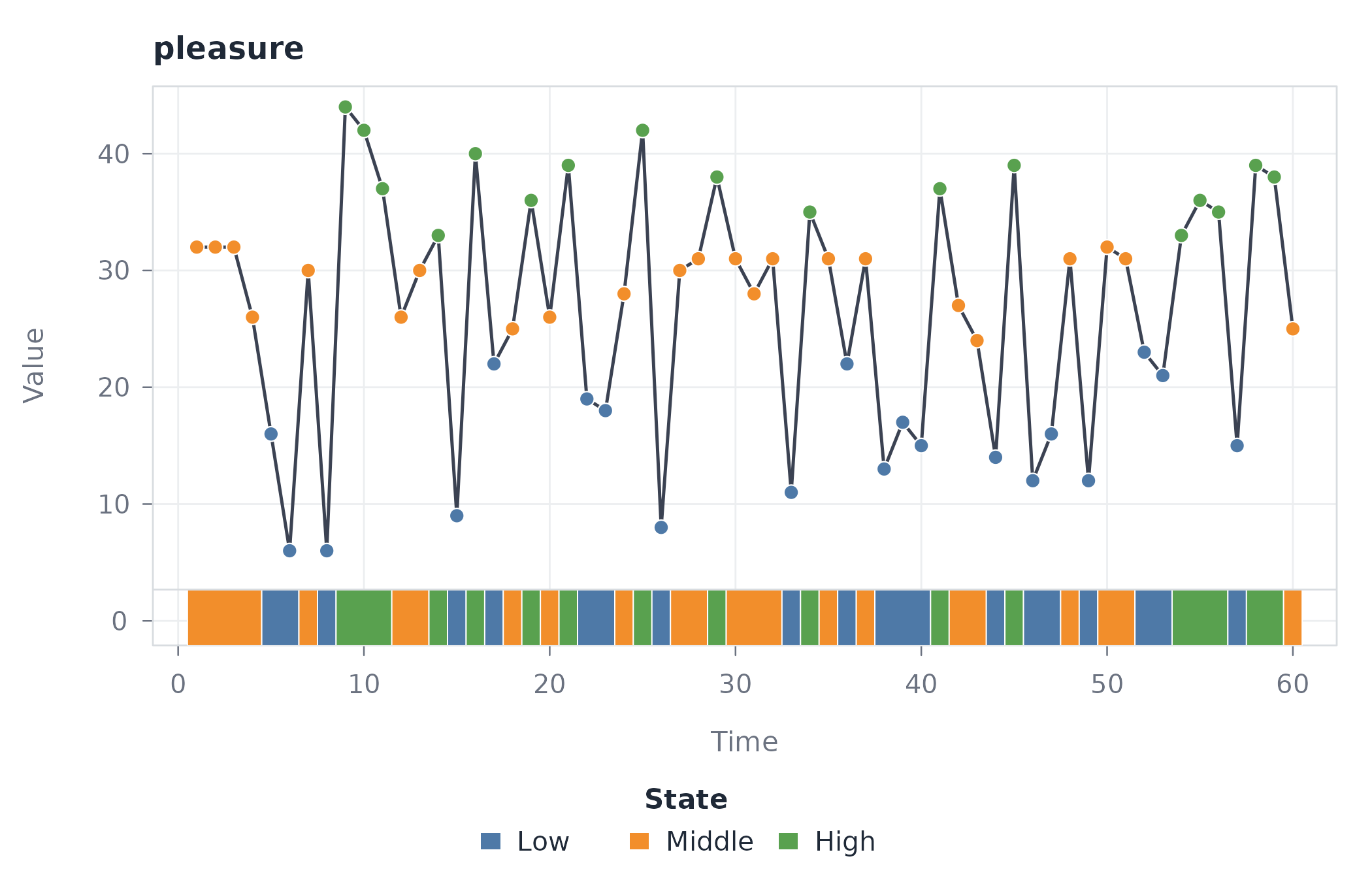

The ribbon places the state encoding outside the measurement panel. It is preferable when vertical shading would conceal short-range variation.

Heatmap

plot(states, "heatmap")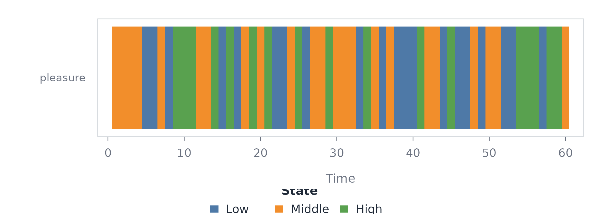

Each tile represents one time point and its colour represents the assigned state. For one series, the result is a compact categorical timeline.

Stack

The stack view is appropriate when states are defined from a transformation of the measured series. Here, one-step changes are discretized and plotted beneath the original observations.

changes <- with(pleasure, c(0, diff(pleasure)))

change_states <- discretize(
  data = changes,
  labels = c("Negative", "Stable", "Positive")
)

plot(
  change_states,
  "stack",
  with = with(pleasure, pleasure),
  with_label = "Pleasure"
)

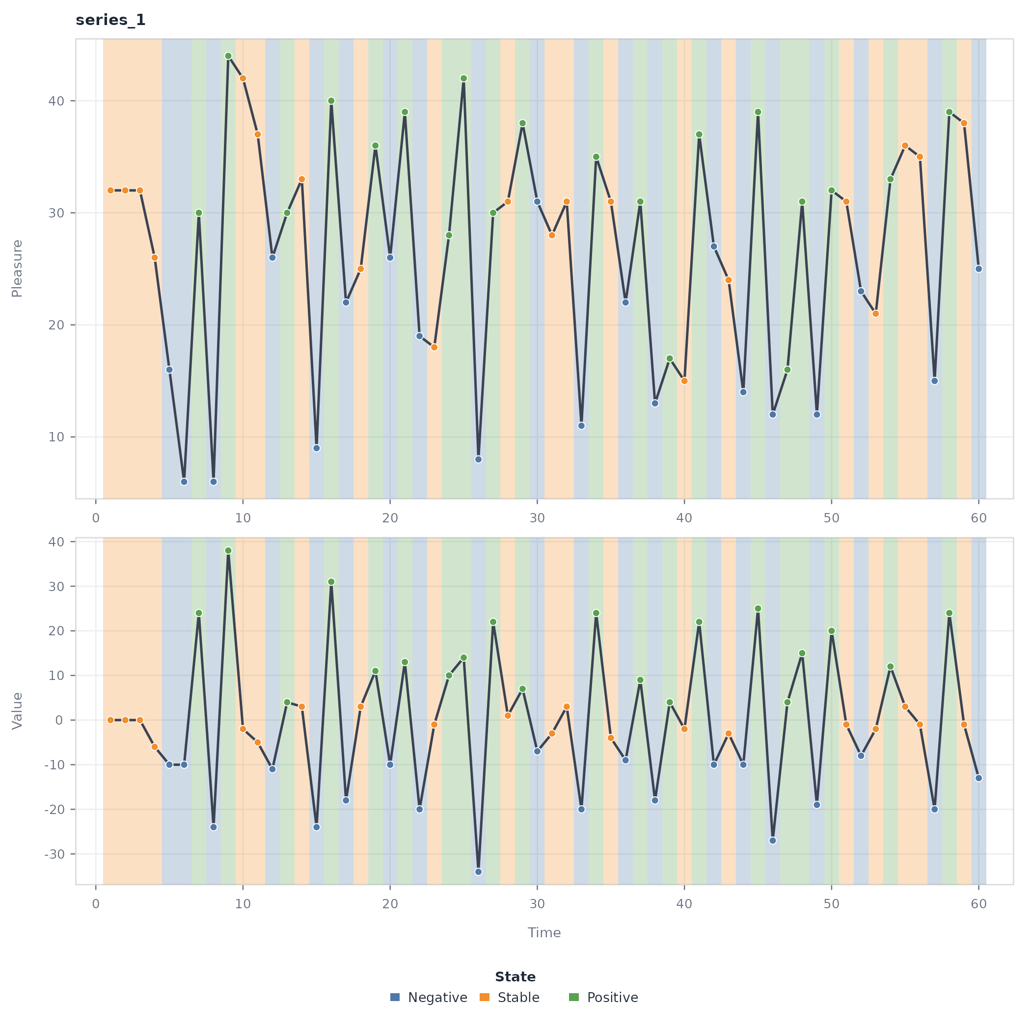
The shared time axis permits changes in the original measurement to be read directly against their categorical representation.

Local-direction plots

The plot() method for a tsn_trend object provides four views of the rolling direction classification.

type	Graphical encoding	Scientific use
"points"	Observations coloured by direction	Locating ascending, descending, flat, and turbulent intervals
"ribbon"	Direction strip beneath the measured series	Separating classification from measurement variation
"heatmap"	Categorical direction tiles	Summarizing the timing of local direction
"panels"	Measured series above the rolling trend metric	Diagnosing how the numerical metric produces the classification

The common arguments series, palette, legend, and grid control selection and presentation. The line and point encodings are modified with line_color, line_width, and point_size. In the panel view, flat_band controls whether the classification threshold is shown. Heatmap presentation can be modified with sort and border.

Points

The local-direction model is fitted and immediately plotted using its default point representation.

directions <- trend(
  data = pleasure,
  series = "pleasure"
)

plot(directions)

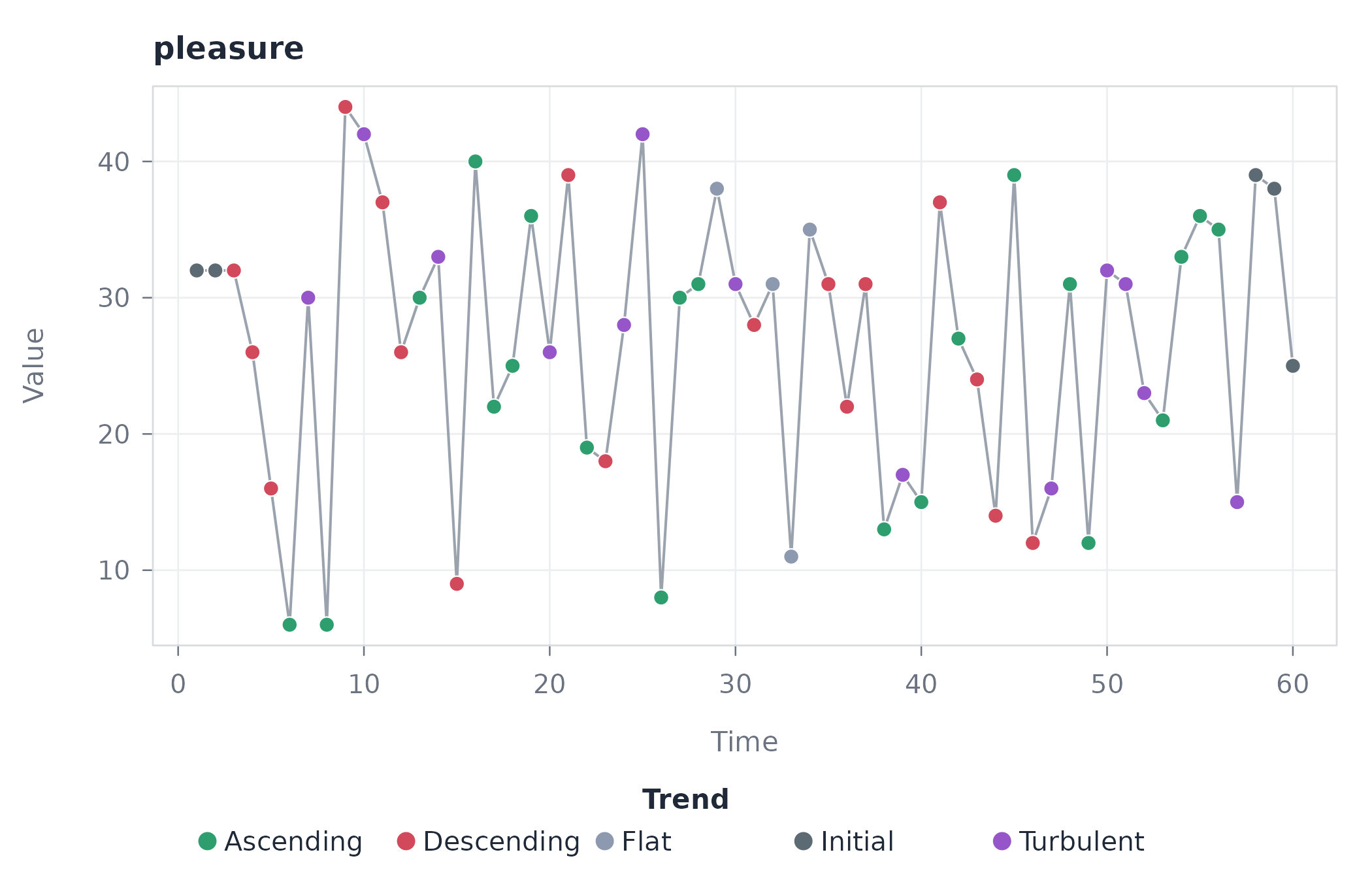
Colour encodes the local trend state at each observation: ascending, descending, and flat record the direction of the window centred on that point, while turbulent marks intervals too volatile to read as a single direction. The view retains individual measurements and is therefore suited to locating directional changes precisely in time.

Ribbon

plot(directions, "ribbon")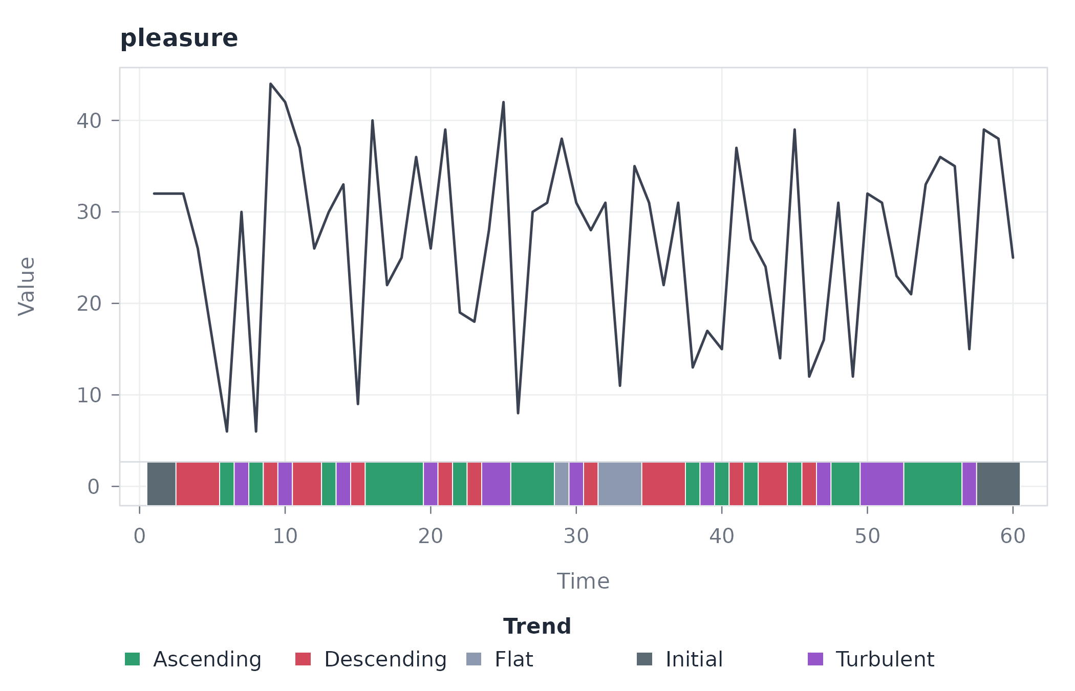

The ribbon is useful when adjacent classifications change frequently, because the measured line remains visually continuous.

Heatmap

plot(directions, "heatmap")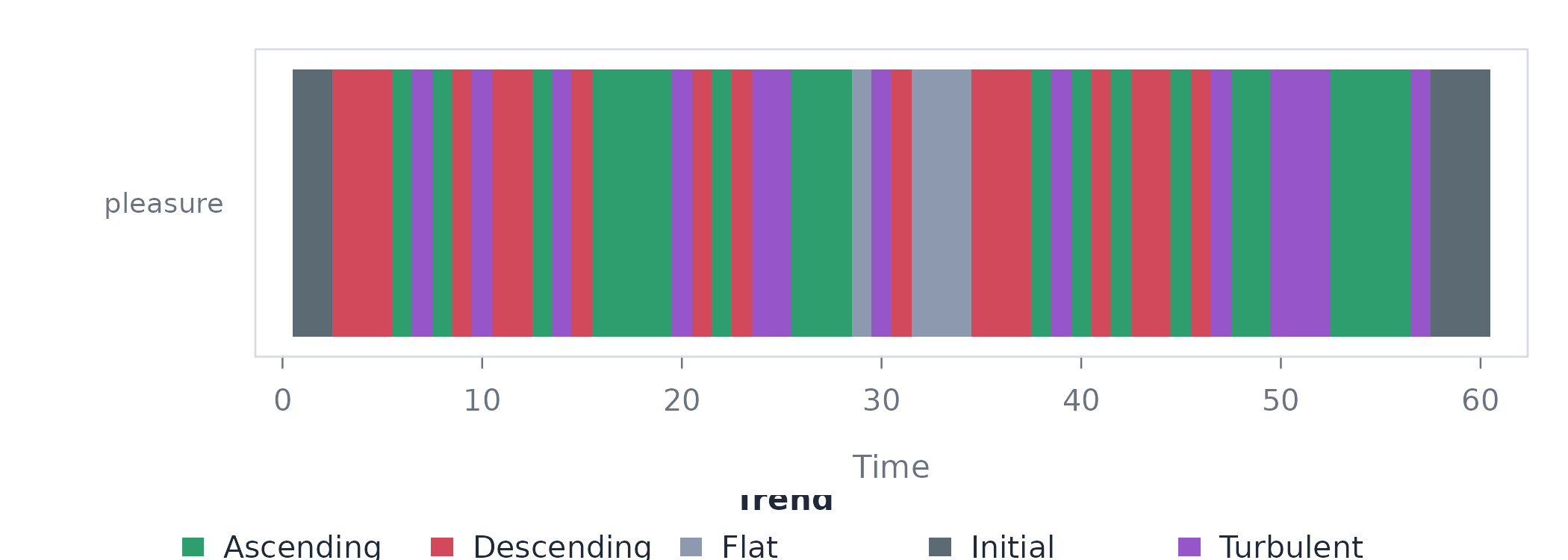

The heatmap removes magnitude and preserves only temporal classification. It should therefore be interpreted as a map of direction, not as a plot of the observed values.

Panels

plot(directions, "panels")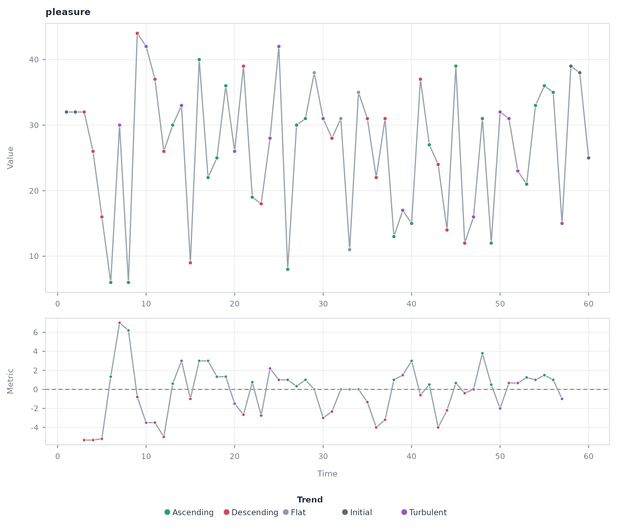

The lower panel displays the rolling metric used to assign direction. This is the appropriate diagnostic view for evaluating crossings of the flat band and their correspondence with the measured series.

Constructed-network plots

Objects returned by tsn() and vg() provide two plot types.

type	Graphical encoding	Scientific use
"network"	Nodes and edges of the constructed network	Examining relational structure, central observations, and connectivity
"series"	Measurements retained in the network object	Verifying the temporal data from which the network was constructed

For type = "network", graphical arguments are passed to cograph::splot(). Important options include layout, labels, node_size, node_fill, edge_color, and edge-label controls. The tsn defaults use a spring layout, degree-based node sizing, and unobtrusive edge styling. For type = "series", arguments such as overlay, points, trend, legend, and grid modify the temporal view.

Network

A horizontal visibility graph is constructed and immediately plotted. The default type is "network".

visibility <- vg(
  data = short,
  type = "horizontal",
  series = "pleasure"
)

plot(visibility)

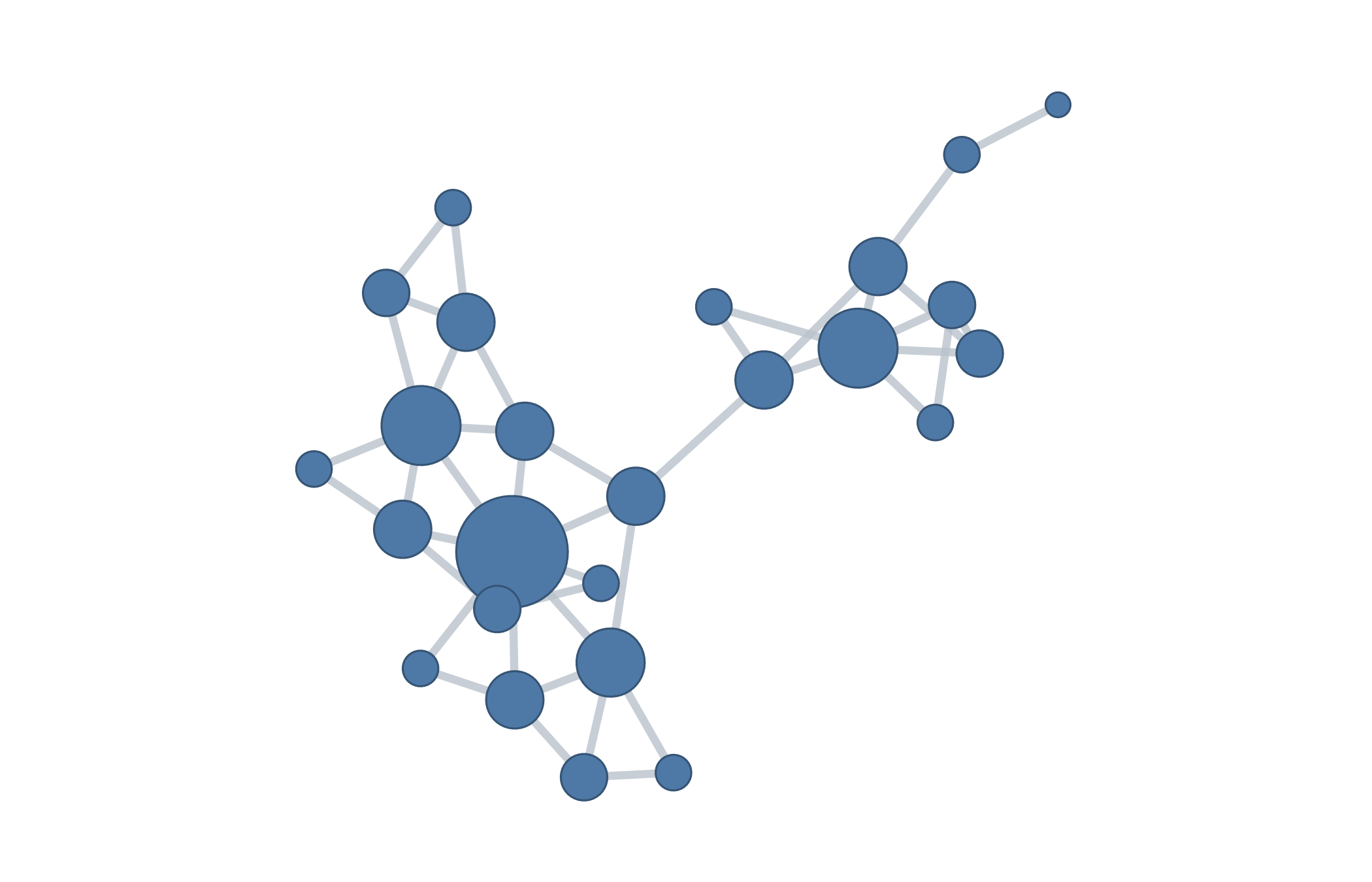
Nodes represent observations and edges represent horizontal visibility. The network view removes the explicit time axis and emphasizes which observations remain mutually visible across intervening values.

Source series

visibility <- vg(
  data = short,
  type = "horizontal",
  series = "pleasure"
)

plot(visibility, "series")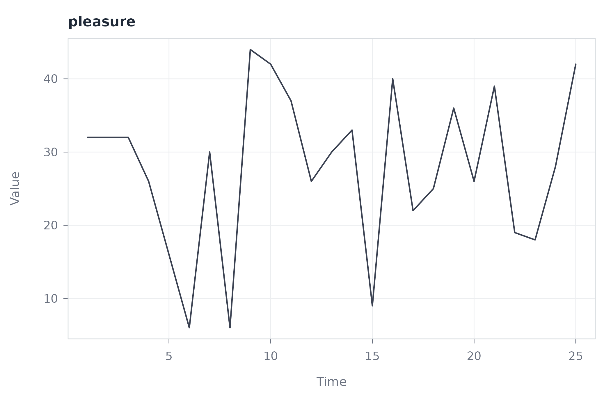

The source-series view restores magnitude and temporal order. It is a diagnostic complement to the network rather than an alternative network model.

Weighted distance network

The visibility graph above is unweighted: an edge is either present or absent. tsn() with method = "distance" instead joins sliding windows of the series and assigns each edge a weight equal to 1 / (1 + distance), so the same "network" plot type now carries continuous structure. The connect = "nearest" rule retains only each window’s two nearest neighbours, which keeps the figure legible.

windows <- tsn(
  data = short,
  method = "distance",
  series = "pleasure",
  step = 2,
  connect = "nearest",
  neighbors = 2
)

plot(windows)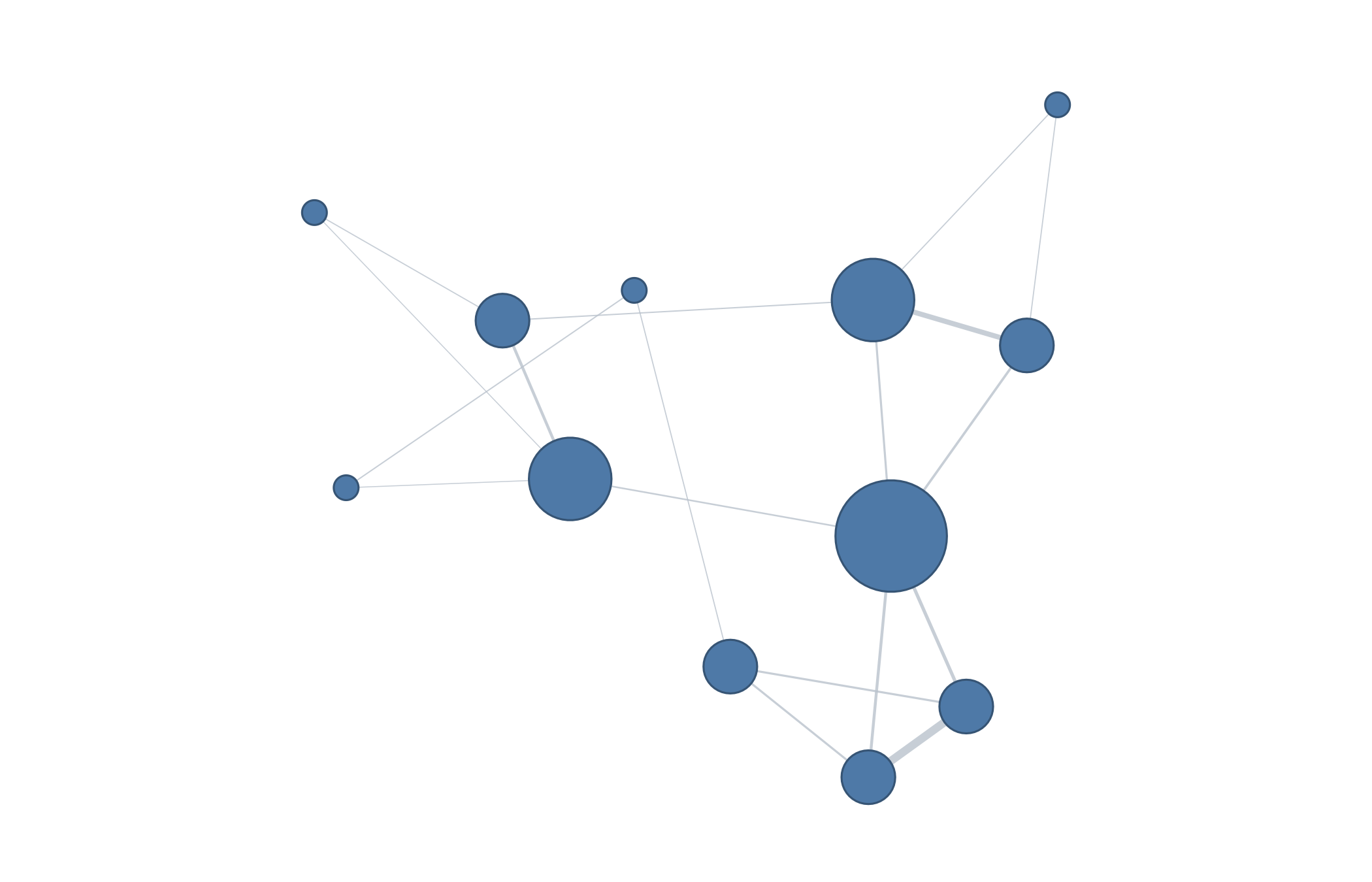

Node size still encodes degree, but the edges now express graded similarity rather than presence alone. The same plot type therefore reports a different kind of structure once the underlying model changes from visibility to distance: the constructor, not the plot argument, determines what an edge means.

Adjusting the network encoding

Graphical arguments change how a network is drawn without changing the fitted object. Here the visibility graph is redrawn with a circular layout; the nodes, edges, and weights are identical to the default view above.

visibility <- vg(
  data = short,
  type = "horizontal",
  series = "pleasure"
)

plot(visibility, layout = "circle")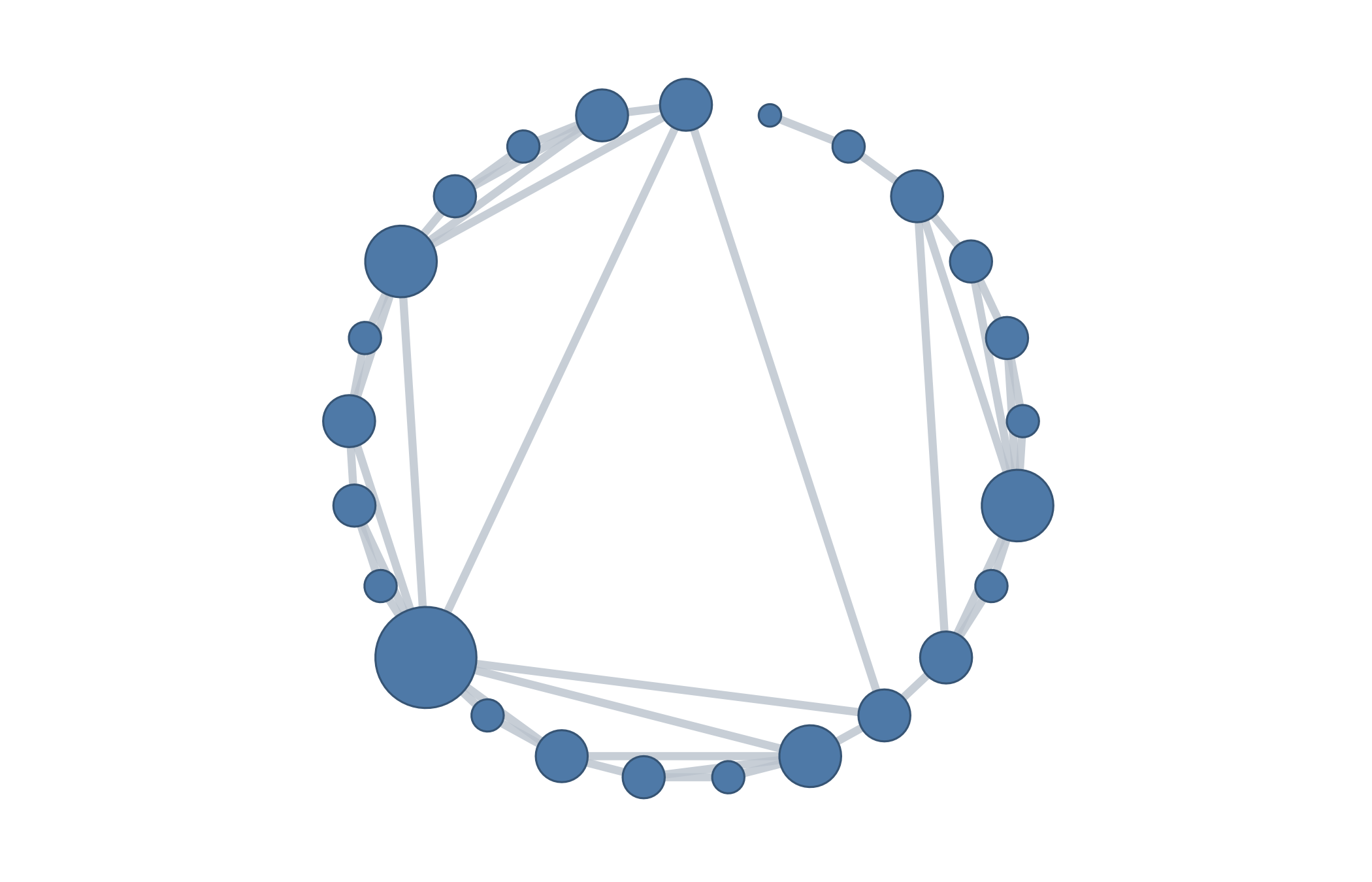

The circular layout places the observations evenly around a ring, but the graph itself is unchanged. This separation matters for interpretation: a claim about central or peripheral observations must rest on the edges stored in the model, not on the visual prominence a particular layout happens to give a node.

Transition Network Analysis plots

The TNA family comprises models returned by ts_tna(), ts_ftna(), ts_cna(), and ts_atna(). Each model supports the same three plot types.

type	Graphical encoding	Scientific use
"combined"	Source sequence and transition network in one figure	Connecting temporal state membership to estimated state relationships
"network"	Transition network only	Examining edge weights, direction, and persistence
"series"	State-classified source sequence only	Inspecting the sequence used to estimate transition relationships

The type argument selects the overall representation. Within the combined view, network_width controls the relative width of the network panel. overlay and ribbon determine how states are displayed with the source series, while points, alpha, and palette control its appearance. Network encoding is modified with node_size, node_scale, and show_weights. Arguments not consumed by the tsn method are passed to cograph::splot().

The network argument selects a per-series or summary network. These coincide for the single source series used here. The distinction becomes relevant only when a model contains more than one source sequence.

Combined

The state sequence is converted to a transition network and immediately plotted. The combined representation is the default.

probabilities <- ts_tna(states)

plot(probabilities)

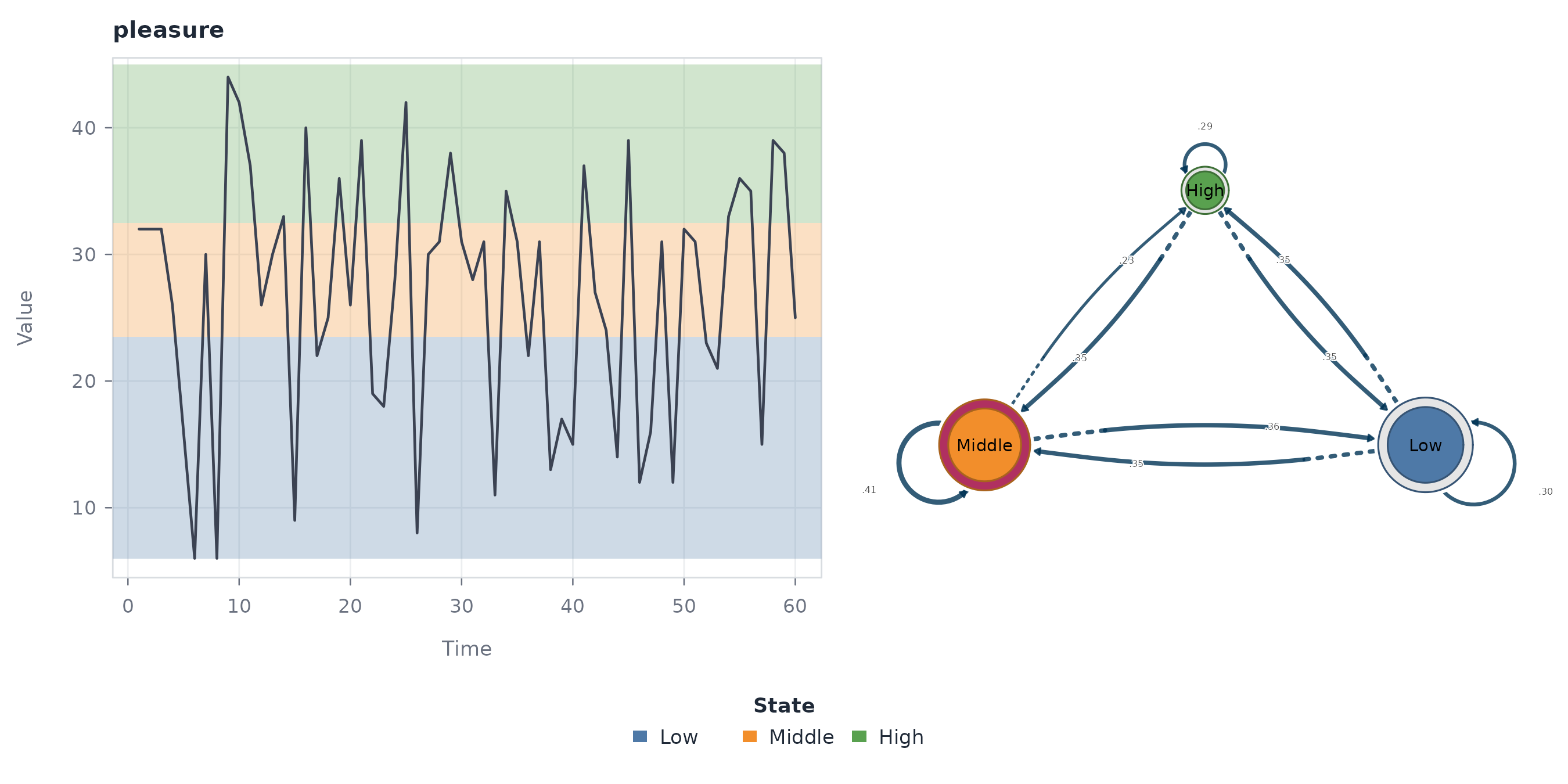
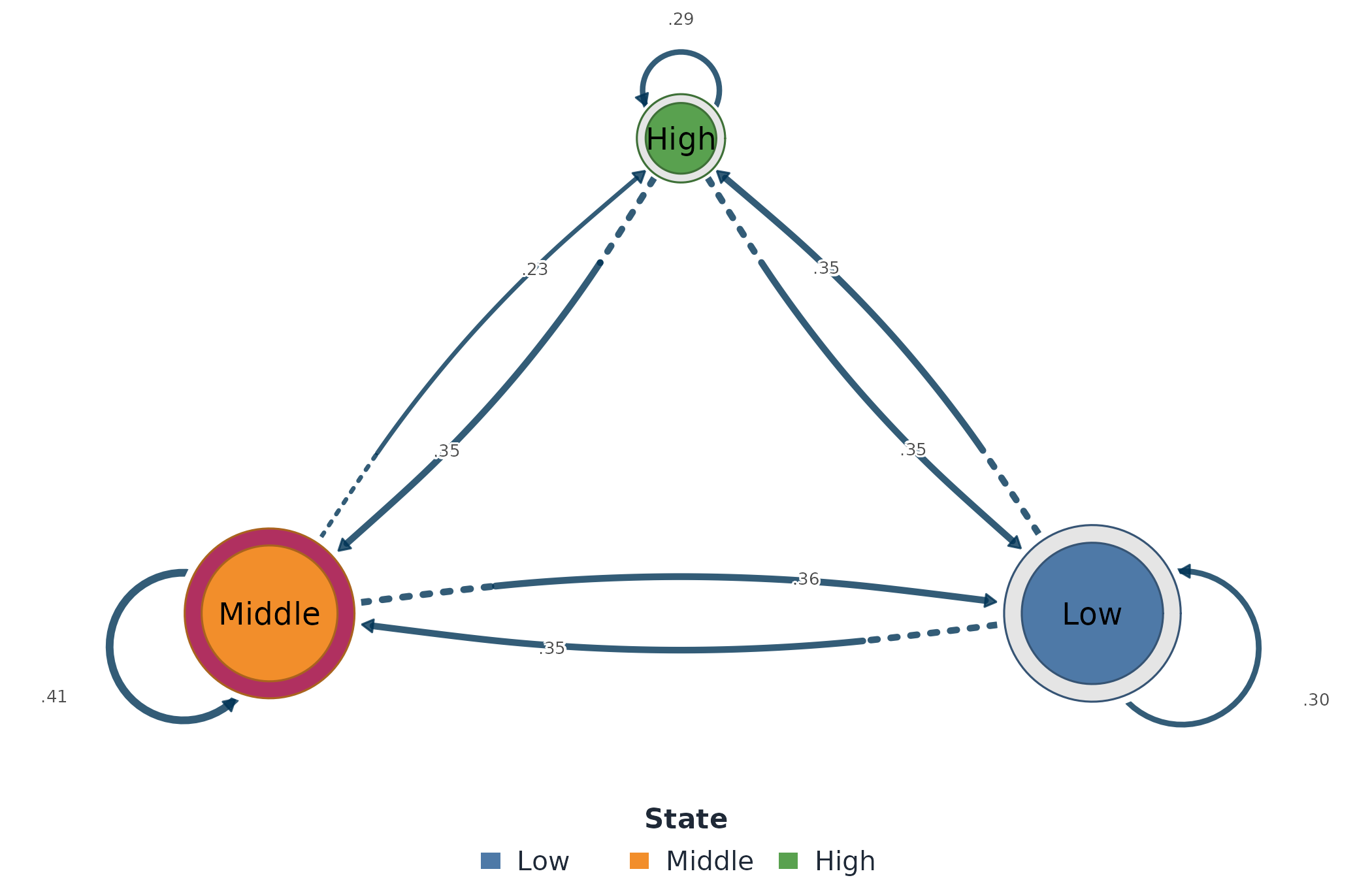
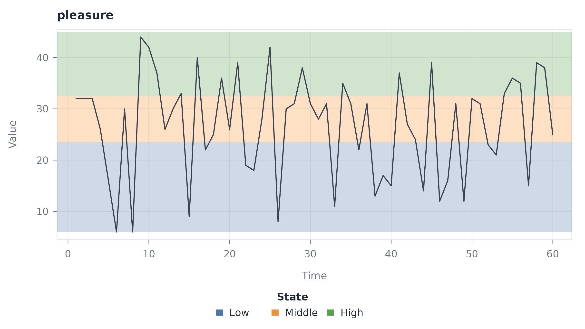
The temporal panel preserves the observations and their assigned states. The network panel represents states as nodes and conditional transition probabilities as directed edges. Their juxtaposition makes the derivation of the relational structure explicit.

Network

probabilities <- ts_tna(states)

plot(probabilities, "network")

The network-only view allocates the full plotting region to the relational structure. Directed edges encode conditional transition probabilities and self-loops encode persistence.

Source series

probabilities <- ts_tna(states)

plot(probabilities, "series")

The series-only view retains the state classification but suppresses the network. It is used to inspect the sequence from which transition weights were estimated.

Extracted-model plots

series_networks() creates an indexed collection of source-specific network models. Its series argument selects a model when the collection contains more than one source. With the single series used here, no selection argument is required. The model is extracted and plotted in the same code block.

probabilities <- ts_tna(states)
individual <- series_networks(probabilities)

plot(individual)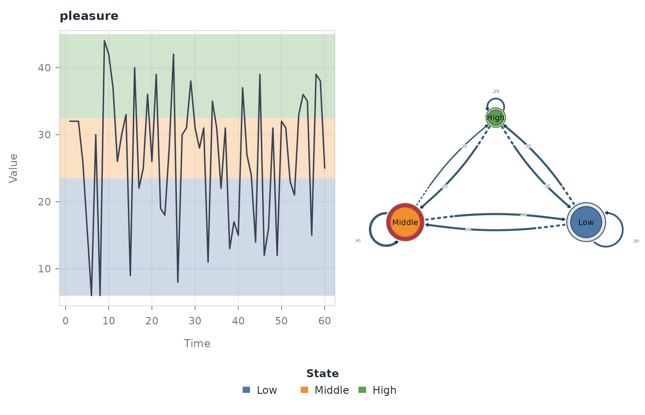

The plot uses the TNA network representation and retains the provenance stored by series_networks().

Selecting a plot

The plot type should follow the scientific question rather than the desired appearance alone.

Scientific question	Recommended view
When do discrete states or local directions occur?	State overlay, ribbon, or trend points
How was a classification produced?	Trend panels or a stacked state view
What temporal sequence generated the network?	Source-series view
What relationships define the constructed network?	Network view
How does a state sequence relate to its transition structure?	Combined TNA view

Arguments controlling colour, size, labels, and layout change the graphical encoding but do not change the fitted object. Consequently, interpretive claims should follow the construction method and edge definition stored in the model, not the visual prominence created by a particular style option.