Plot a simulated bootstrap null distribution

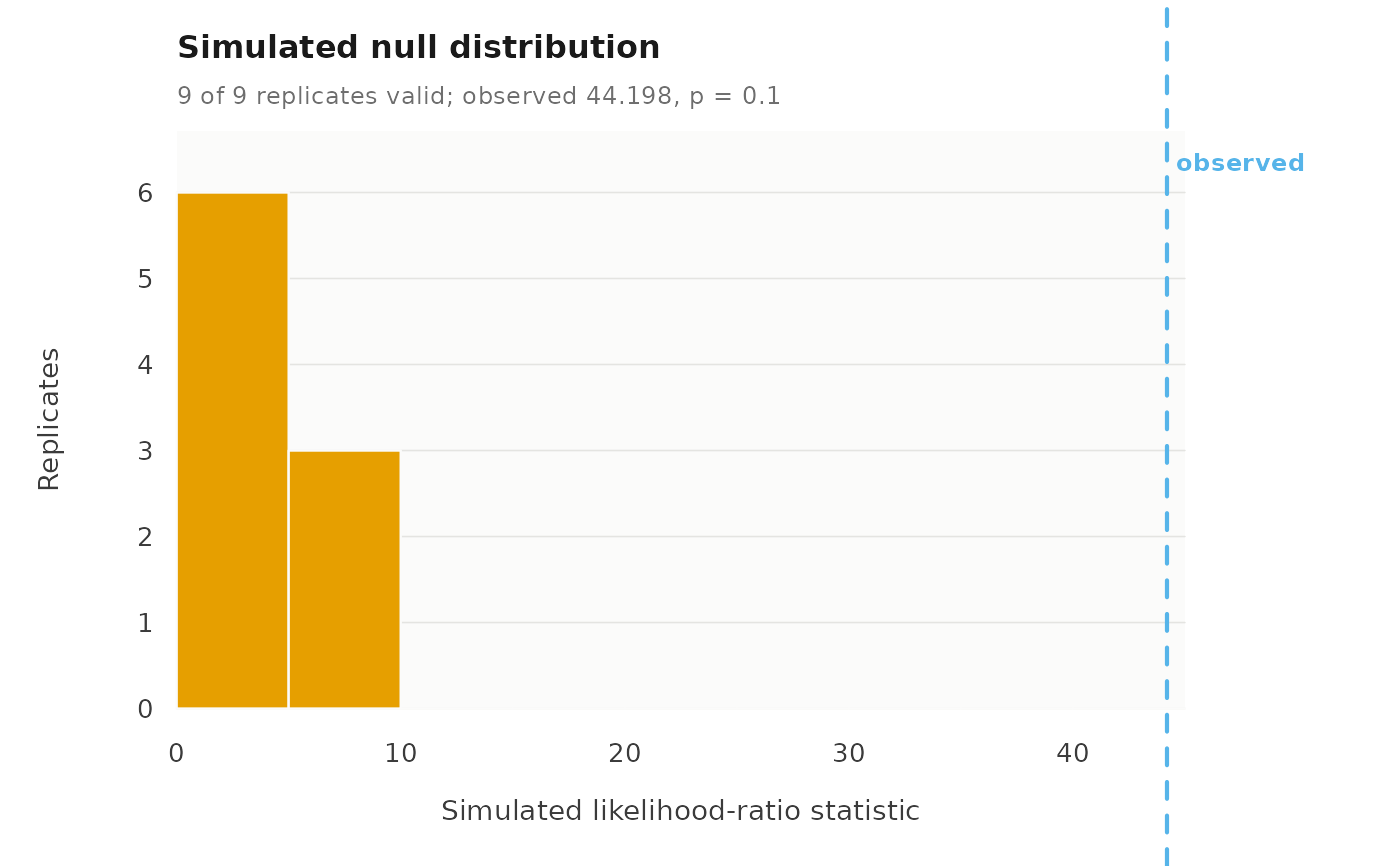
Draws the replicate likelihood-ratio statistics as a histogram with the observed statistic marked, so that the p-value can be read as a tail area of the distribution that was actually simulated. Invalid replicates carry no statistic and are counted in the subtitle rather than dropped silently.

Usage

# S3 method for class 'multilpa_bootstrap_lrt'
plot(
  x,
  main = NULL,
  subtitle = NULL,
  palette = NULL,
  style = .multilpa_style(),
  ...
)

Arguments

x

An multilpa_bootstrap_lrt result.

main, subtitle

Panel title and secondary line, or NULL for defaults.

palette

A vector of at least two colours: the histogram fill and the observed-statistic marker. NULL uses the package palette.

style

A list of visual constants, as built by .multilpa_style().

...

Further named visual constants, merged into style.

Value

The input, invisibly. Called for the side effect of drawing.

Conditions

latents_nothing_to_plot when no replicate produced a finite statistic.

Examples

set.seed(1)
example_data <- data.frame(
  school = rep(seq_len(10), each = 10),
  score = rnorm(100, rep(c(-2, 2), each = 50))
)
smaller <- multilpa(example_data, "score", "school", n_profiles = 1,
                    n_group_classes = 1, n_starts = 2, seed = 1)
larger <- multilpa(example_data, "score", "school", n_profiles = 2,
                   n_group_classes = 1, n_starts = 2, seed = 1)
# `iter` is small so the example runs quickly; use many more for inference.
comparison <- bootstrap_lrt(smaller, larger, iter = 9, n_starts = 1,
                            max_iter = 2000, tol = 1e-6, seed = 1)
plot(comparison)