Plot a fitted multilevel latent profile model

Draws one view of a fit as a ggplot object, which can be printed, saved with ggplot2::ggsave() or styled further with + ggplot2::theme(). Every view shares one profile order (largest first), one profile share (the posterior share every table reports) and one set of Okabe-Ito colours paired with point shapes, so a profile looks the same in every view. Series are labelled directly rather than through a legend.

Usage

# S3 method for class 'multilpa'
plot(
  x,
  what = c("profiles", "bars", "heatmap", "raincloud", "parallel", "pairs", "responses",
    "probabilities", "sequences", "sizes", "entropy", "posteriors", "avepp", "all"),
  data = NULL,
  scale = c("raw", "standardized"),
  category = "last",
  labels = TRUE,
  intervals = TRUE,
  cell_labels = TRUE,
  main = NULL,
  subtitle = NULL,
  statistic = c("mean", "median", "mode"),
  ...
)

Arguments

x

A fitted multilpa model.

what

Which view to draw. plot_views() lists every value with its group and a one-line description.

The measurement model: "profiles" draws one line per profile across the continuous indicators, or numeric categorical summaries when there are no continuous indicators (see statistic). "bars" draws continuous means as grouped bars that start at zero. "heatmap" draws them as a diverging grid of observed standard deviations from each indicator's observed mean, the quickest read when there are many indicators or profiles; for a fit whose indicators are all categorical it draws the response probabilities instead. "raincloud" shows what the means summarize: for the cases assigned to each profile, a density, the quartiles and the observations of each indicator. "parallel" draws every case as a line across the indicators, one panel per profile, faded by the certainty of its assignment. "pairs" draws a scatter-plot matrix of the indicators with each profile's 95% ellipse from the fitted covariances, the view that shows the covariance structure. "responses" is the categorical counterpart of "profiles": one line per profile, showing the probability of a chosen category.

The two-level structure: "probabilities" plots profile prevalence within each group class. "sequences" draws one row per group and one column per position, filled with the assigned profile; it needs a fit made with time =.

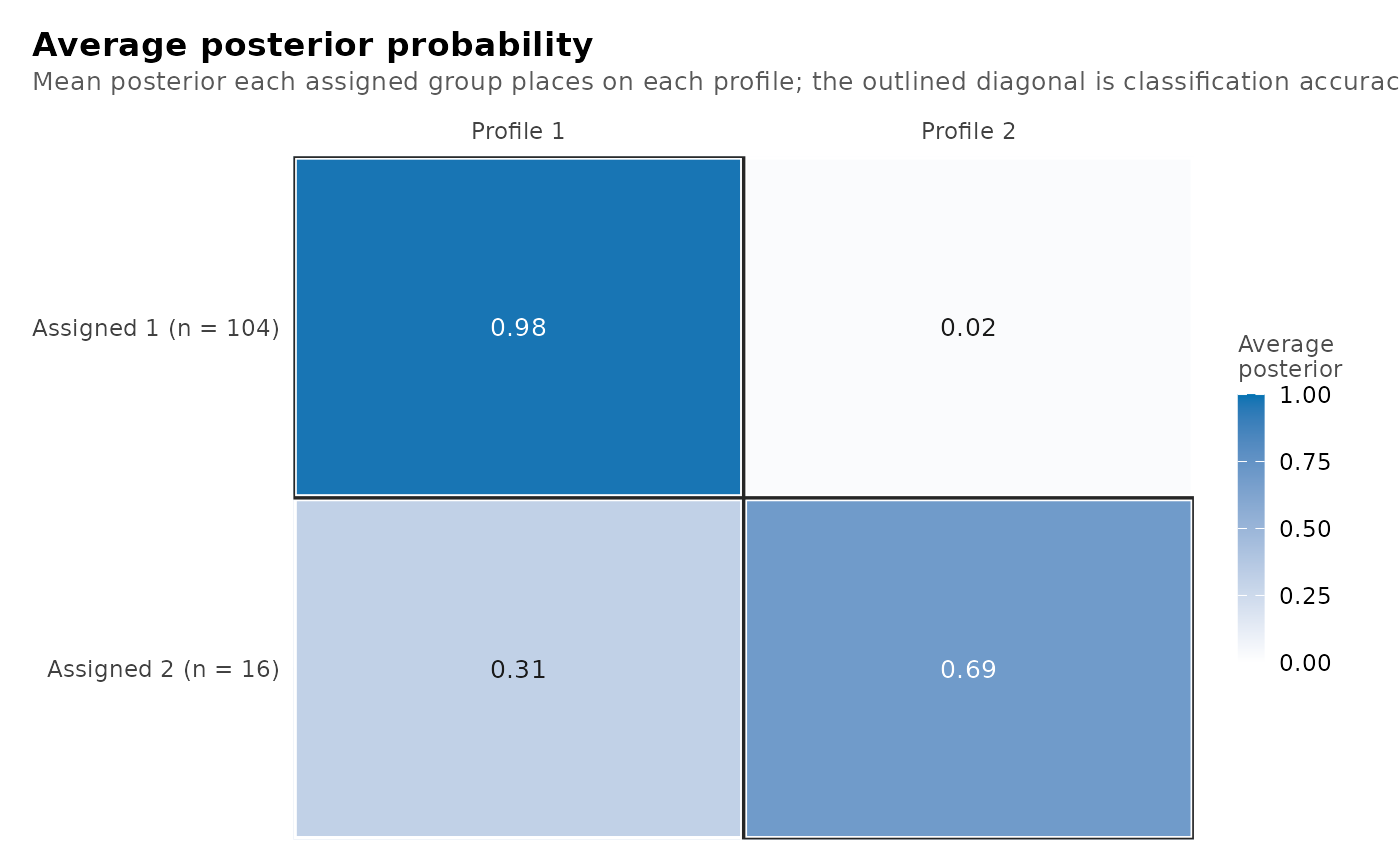
Classification: "sizes" draws each profile's effective count, the posterior mass it carries. "posteriors" draws the posterior probability of each case's assigned profile and "entropy" each case's entropy relative to a flat posterior, one strip per profile with its mean marked. A one-profile fit refuses both with an error of class latents_nothing_to_plot. "avepp" draws the average posterior probability matrix: rows are assigned profiles, columns profiles, and the diagonal is the avePP usually reported.

"all" returns every view the fit has the ingredients for.

data

Optional. The data frame the model was fitted to. A fit carries the columns it was built from, so intervals are drawn without it; pass it only to compute them from a different frame.

scale

For the mean views and "raincloud", "raw" keeps each indicator in its input units and "standardized" divides its deviation from the observed mean by its observed standard deviation, the same map as as.data.frame(scale = "standardized").

category

For what = "responses", which category's probability to plot: "last", "first", or a single category label or index.

labels

TRUE labels each series at its right end; FALSE uses a legend instead.

intervals

For "profiles" and "responses", TRUE draws 95% intervals when the fit has standard errors (a probability's is clipped to [0, 1]). A fit without them is drawn without whiskers and its subtitle says why.

cell_labels

For what = "sequences", TRUE prints the profile number in each cell while the grid is sparse enough to hold one, so the profile is not carried by colour alone.

main, subtitle

Title and subtitle. NULL uses the view's own.

statistic

For what = "profiles", "mean" (default), "median" or "mode". With continuous indicators these are the same fitted Gaussian location. When there are no continuous indicators, summarizes each categorical indicator's fitted probabilities on its numeric category scale. Means assume meaningful score spacing; medians are the smallest score with cumulative probability at least 0.5; tied modes use the smallest score. Category labels must be distinct finite numeric scores. Categorical summaries support only scale = "raw" and have no confidence intervals; they do not run parameter inference. Mixed models retain continuous-only profile plots; use "responses" for their categorical indicators.

...

Nothing further is accepted; an unknown argument raises an error of class latents_bad_argument. Style the returned plot with ggplot2.

Value

A ggplot object; for what = "all", a latents_plots list of them, named by view, that draws every one when printed.

Details

The plots need the ggplot2 package, which latents suggests rather than requires; without it a plot is refused with an error of class latents_missing_package.

"profiles" and "bars" draw 95% Wald intervals when the fit has standard errors. Profile numbers are arbitrary, so two fits must have their labels aligned before their plots are compared. With scale = "standardized" the standard deviations are the observed indicator standard deviations, not the within-profile ones, so the values are comparable across indicators but are not effect sizes.

Errors

latents_missing_package without ggplot2; latents_no_continuous, latents_no_categorical, latents_no_time and latents_nothing_to_plot when the fit lacks what a view needs; latents_bad_argument for an argument the method does not use.

References

Zappia, L. and Oshlack, A. (2018). Clustering trees: a visualization for evaluating clusterings at multiple resolutions. GigaScience, 7(7), giy083.

Examples

if (requireNamespace("ggplot2", quietly = TRUE)) {
  set.seed(7)
  example_data <- data.frame(
    school = rep(seq_len(12), each = 10),
    score_a = rnorm(120), score_b = rnorm(120)
  )
  fit <- multilpa(example_data, c("score_a", "score_b"), "school",
                  n_profiles = 2, n_group_classes = 1, n_starts = 2)
  plot(fit)
  plot(fit, scale = "standardized")
  plot(fit, what = "bars")
  plot(fit, what = "pairs")
  plot(fit, what = "avepp")
}