Plot an LSA Fit

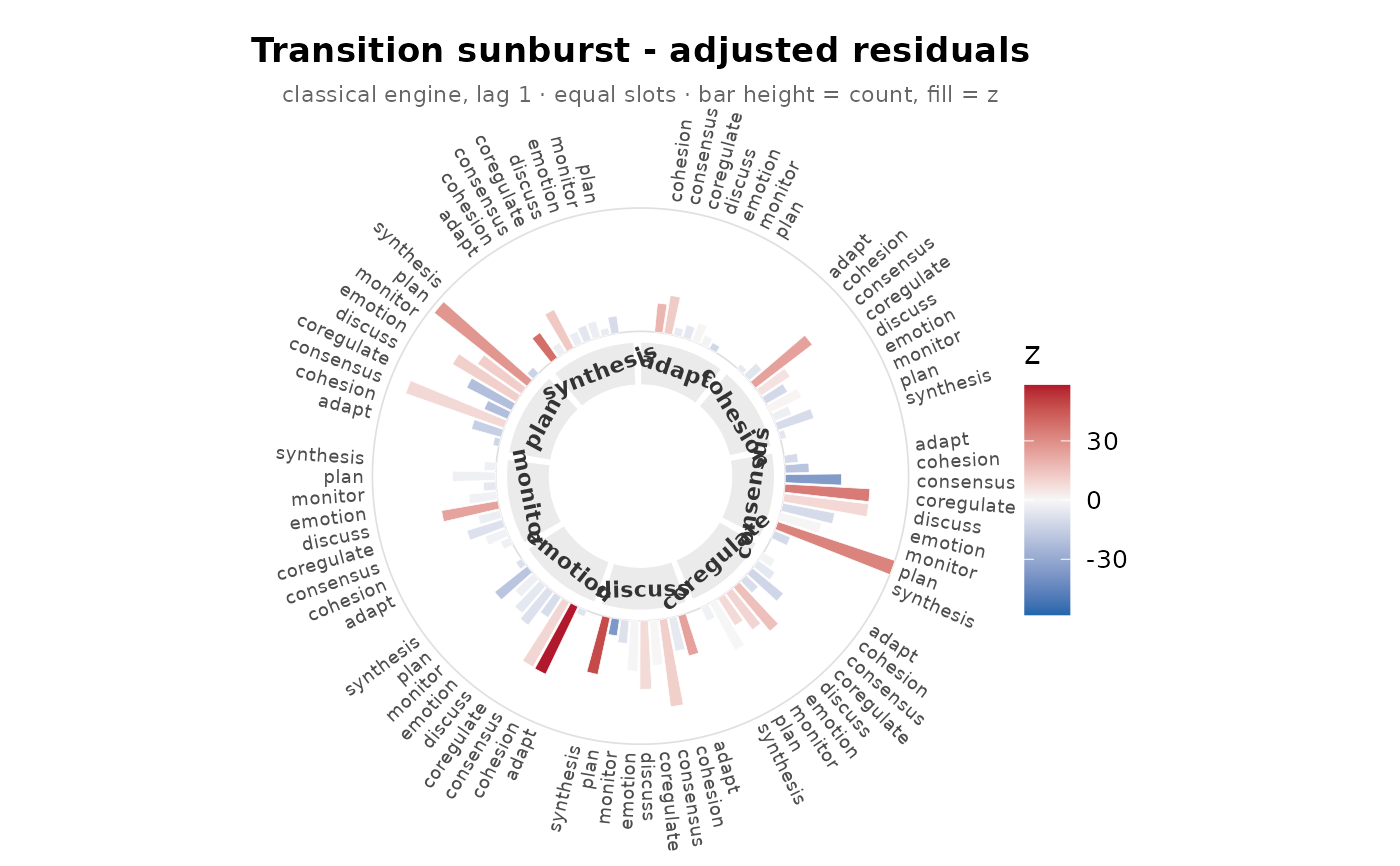
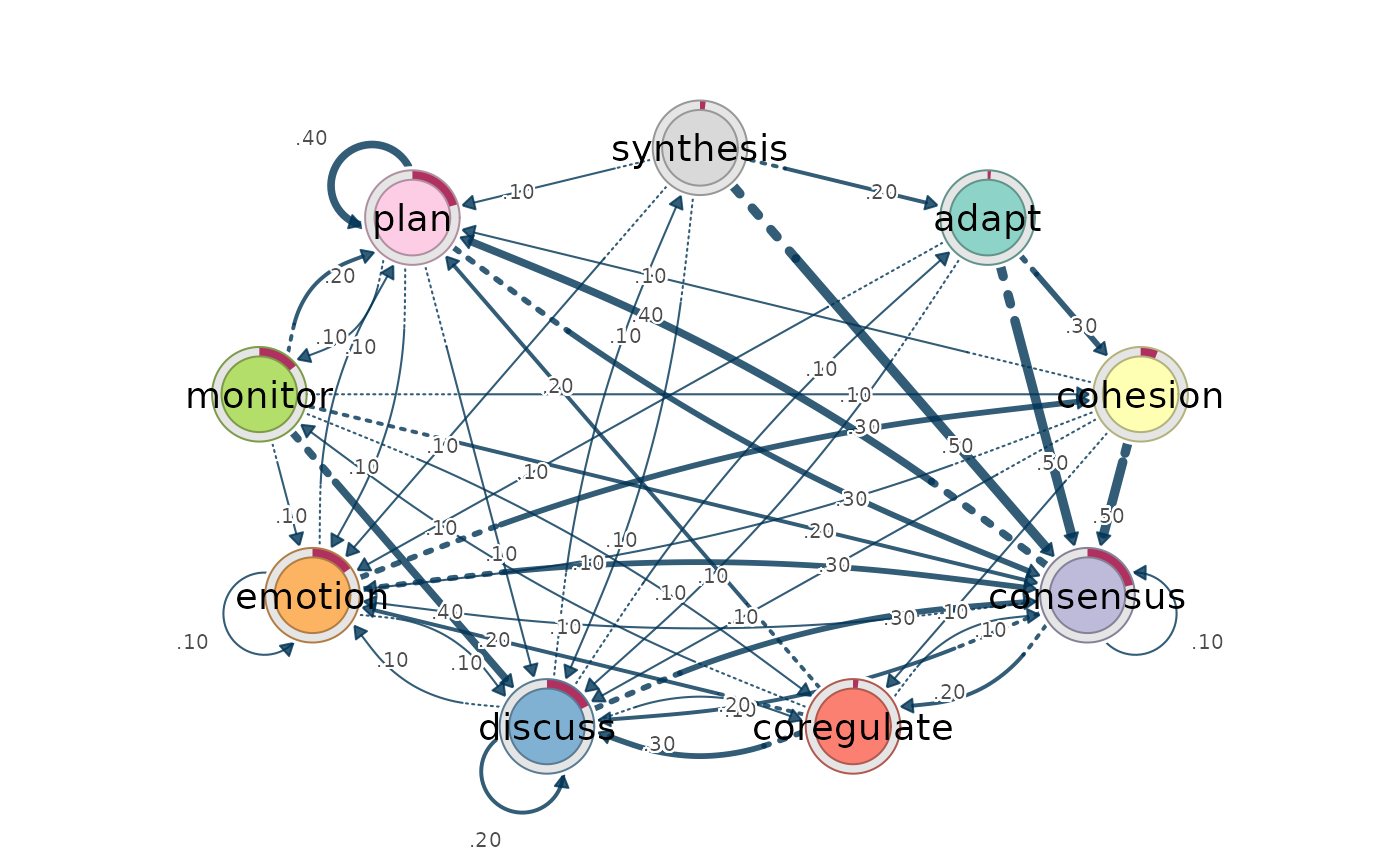
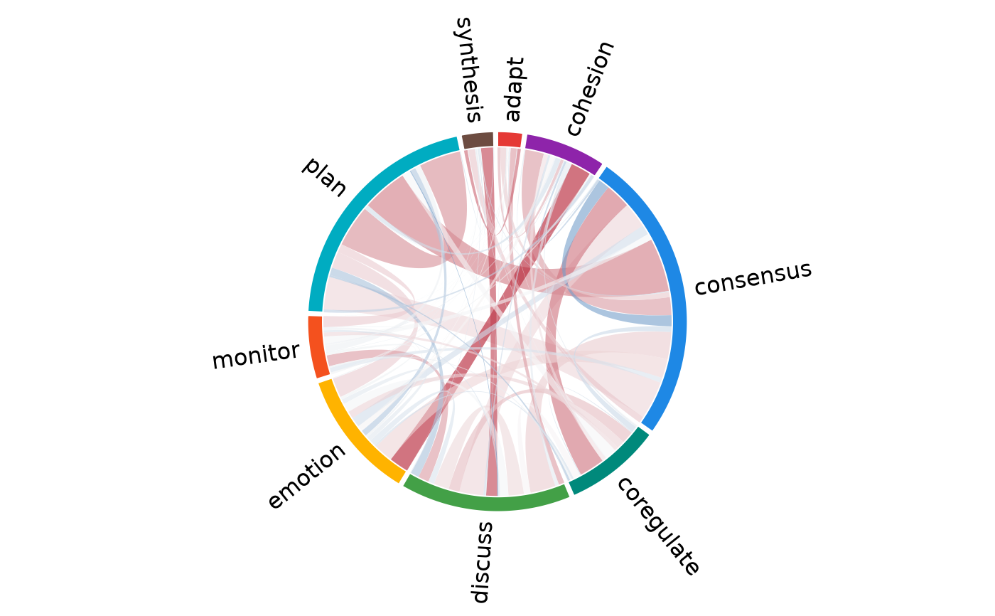
One entry point for every view of a fit; pick it with type: "heatmap" (default, the from x to residual heatmap), "network" (transition network via cograph::splot()), "chord" (chord diagram via cograph::plot_chord()), or "sunburst" (polar rose). Extra arguments are forwarded to the chosen view's worker (plot_transitions(), plot_chords(), plot_polar()); see those for view-specific options.

Usage

# S3 method for class 'lsa'
plot(x, type = c("heatmap", "network", "chord", "sunburst"), ...)

# S3 method for class 'lsa_group'
plot(
  x,
  type = c("heatmap", "network", "chord", "sunburst"),
  combined = FALSE,
  ...
)

Arguments

x

An lsa fit from lsa().

type

Which view to draw: "heatmap" (default), "network", "chord", or "sunburst".

...

Forwarded to the chosen view. For "heatmap": which ("residuals" (default), "prob", "count", "expected"). For "network": weights ("tna" for the probability-weighted TNA network). For "chord": width, color. For "sunburst": style, fill.

combined

Logical, for a grouped fit only. FALSE (default) draws each group as its own full-size figure; TRUE tiles all groups into a single figure (compact, but cramped for many groups).

Value

A ggplot object for "heatmap" and "sunburst"; the (invisible) cograph object for "network" and "chord". Drawn when printed.

See also

plot_transitions(), plot_chords(), plot_polar(), plot_forest(), transitions()

Examples

fit <- lsa(group_regulation)
plot(fit)                     # residual heatmap (default)

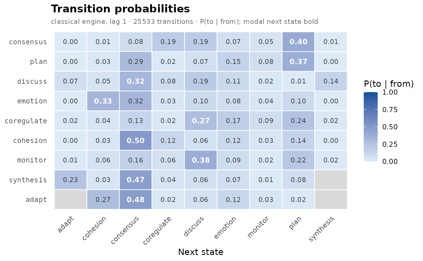
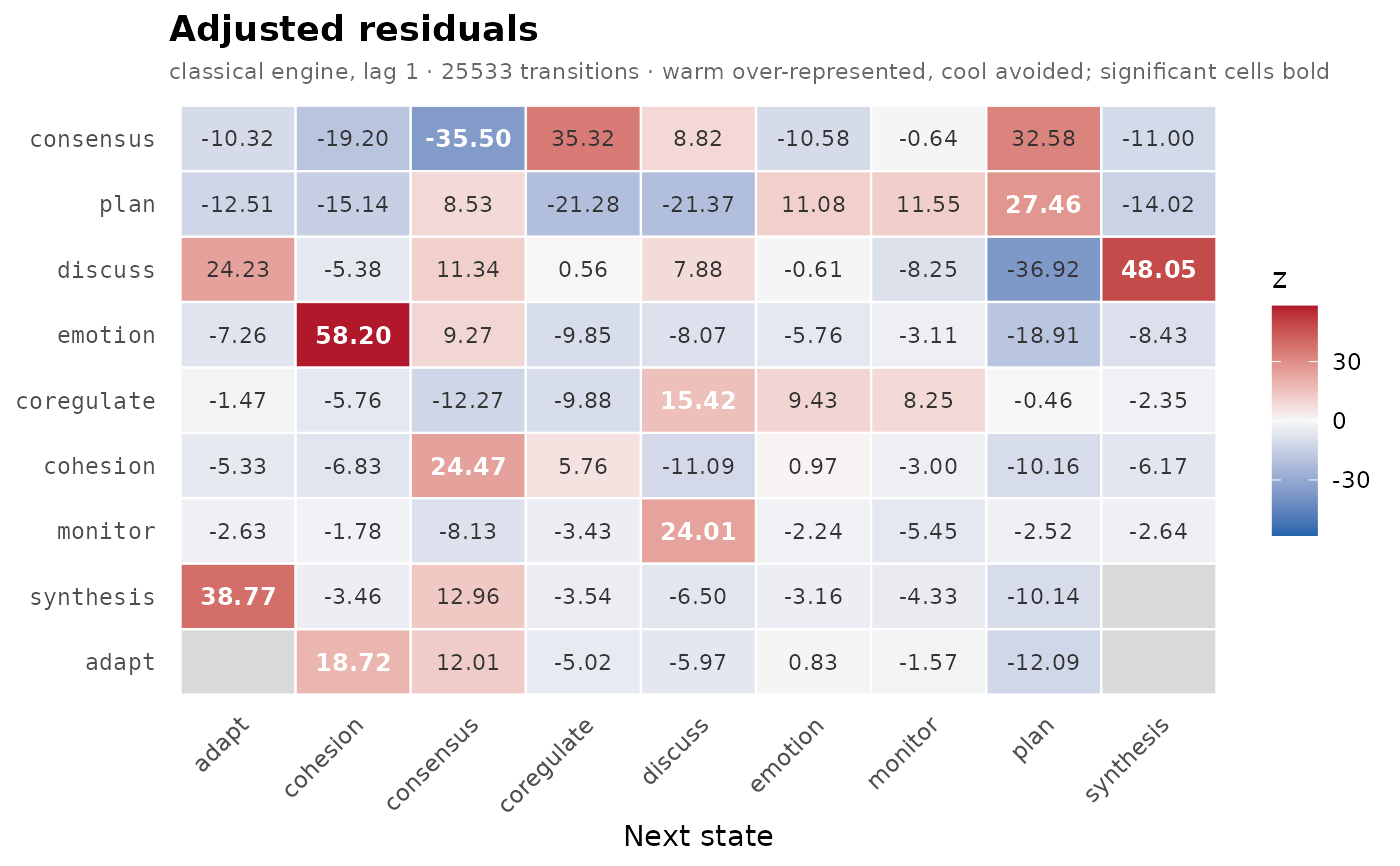plot(fit, which = "prob")     # heatmap of probabilities

plot(fit, type = "network")   # transition network

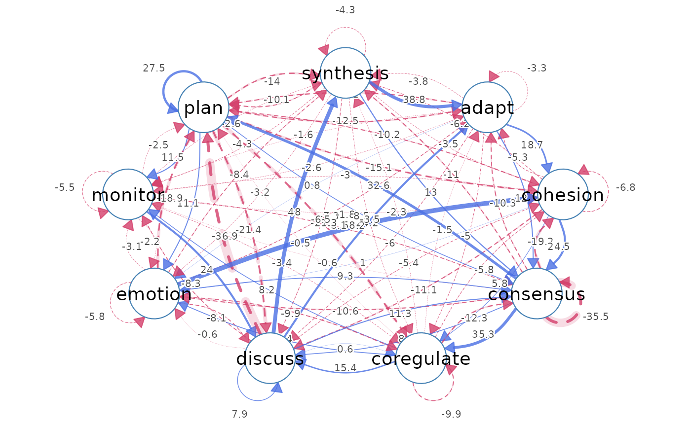plot(fit, type = "network", weights = "tna")  # TNA probability network

plot(fit, type = "chord")     # chord diagram

plot(fit, type = "sunburst")  # polar sunburst