Circular (Chord) Diagram of an LSA Fit

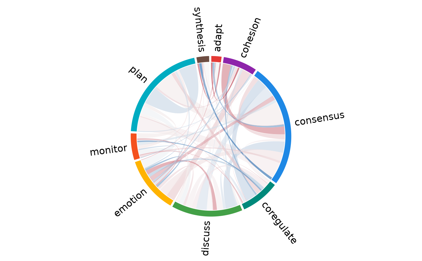
Draws the transition structure as a chord diagram via cograph::plot_chord(): states are arcs on an outer ring and each transition is a curved ribbon whose width is its frequency (or probability) and whose fill colour is its adjusted residual (warm = over-represented, cool = avoided). Supply a second fit as compare to fill each ribbon by the difference in the colour metric between the two fits.

Usage

plot_chords(
  fit,
  compare = NULL,
  width = c("count", "prob"),
  color = c("residuals", "lift", "prob", "count"),
  significant = FALSE,
  self_loops = TRUE,
  alpha = 0.6,
  ...
)

Arguments

fit

An lsa fit from lsa().

compare

Optional second lsa fit. When supplied, ribbon colour is colour(fit) - colour(compare) (a signed difference on the diverging scale). The two fits must share the same states. Default NULL.

width

Which non-negative quantity sets ribbon width: "count" (default, transition frequency) or "prob" (row-conditional probability).

color

Which quantity fills the ribbons: "residuals" (default, signed adjusted residual, diverging), "lift", "prob", or "count". Non-residual metrics use a sequential scale unless compare makes them a signed difference.

significant

Logical. Keep only significant transitions (drops the others' ribbons). Ignored when compare is set. Default FALSE.

self_loops

Logical. Draw self-transition ribbons. Default TRUE.

alpha

Ribbon fill opacity. Default 0.6.

...

Passed to cograph::plot_chord() (e.g. ticks, segment_width, label_size, title).

Value

Invisibly, the list returned by cograph::plot_chord() (segments and chords data frames). Drawn as a side effect.

Details

This is the circular companion to the plot.lsa() heatmap and the plot_transitions() network. Like them it delegates the drawing to cograph; it needs the cograph package installed.

See also

plot.lsa() (heatmap), plot_transitions() (network), transitions()

Examples

fit <- lsa(group_regulation)
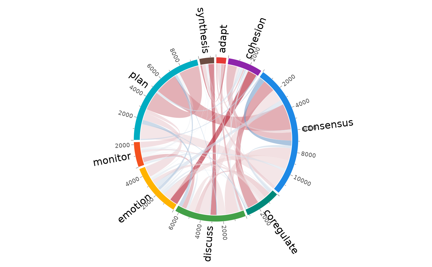
plot_chords(fit)                          # ribbons filled by residual

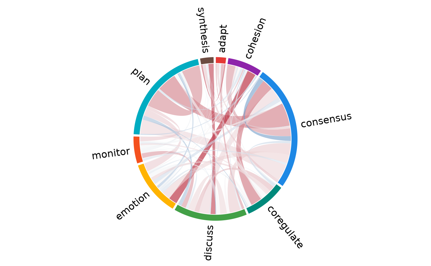plot_chords(fit, width = "prob")          # width = probability

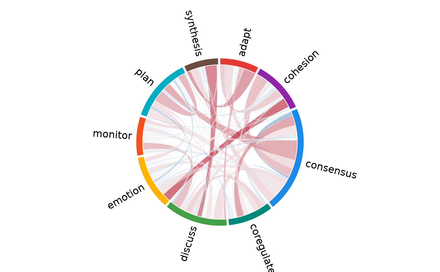plot_chords(fit, significant = TRUE, ticks = TRUE)


# Compare two groups: ribbon colour = difference in residuals.
g <- lsa(group_regulation,
         group = rep(c("A", "B"), length.out = nrow(group_regulation)))
plot_chords(g$A, compare = g$B)