Introduction

Summary

lagdynamics implements lag-sequential analysis (LSA) and its network representation, the lag transition network, for categorical event and sequence data. LSA is the classical inferential method for temporal contingency in observed behaviour: it tests, for every ordered pair of states, whether one state follows another more or less often than independence predicts. The package restates this method as a modern statistical workflow built on six commitments:

Tidy. Every result is produced by a verb – transitions(), nodes(), tests(), initial(), summary(), transition_probabilities() – that returns a one-row-per-observation data frame. transitions() reads the fitted model and every inference result through the same arguments. Filters are arguments (significant = TRUE, direction = "over", min_count =), never subsetting; the user never indexes into an object.
Confirmatory, following Dynalytics. The package operationalizes the Dynalytics framework, whose central tenet is a scientific contract: every analytical claim is matched by evidence appropriate to its structure, scope, and complexity. Validation is therefore expanded far beyond the classical residual test into a full battery – analytic Bayesian certainty, sequence-level bootstrap, split-half reliability, case-drop stability, and a within-sequence permutation null.
Expanded. Beyond the classical engine the package offers five estimation engines plus an open registry for user-defined ones, multi-lag analysis with positive and negative lags, structural-zero constraints under quasi-independence, initial and transition probabilities, grouped estimation in a shared state space, and an experimental directed transfer-entropy measure.
Group-aware. A grouping variable yields one model per group, and group differences are tested rather than eyeballed: compare_lsa() permutes labels over whole sequences and bayes_compare_lsa() gives the analytic Bayesian counterpart, both with multiplicity adjustment and pairwise comparison for more than two groups.
Visual. A large array of plots covers every level of the analysis: residual heatmaps, residual networks, probability-weighted TNA transition networks, chord diagrams, polar sunbursts, uncertainty forests for the bootstrap and certainty results, and group barrels and difference heatmaps for the comparisons.
Interoperable. The package plugs into the other dynamics packages on both sides: lsa() ingests long event logs, wide data, lists of sequences, TraMineR state sequences, tna models and sequence data, and Nestimate prepared data, while the fitted object is a cograph network that cograph renders directly and exposes the transition and initial probabilities that TNA-style tooling consumes.

The numerical core is a clean-room implementation. Every formula was transcribed from its primary source – with page and equation numbers recorded in the package’s formula reference map (inst/REFERENCES.md) – and implemented without consulting any prior LSA software. The implementation is cross-validated against base-R primitives (stats::loglin() for iterative proportional fitting, stats::chisq.test() standardized residuals, stats::binom.test(), stats::pchisq()) and against hand-derived algebraic identities. The analytical core depends only on base R; the plotting functions additionally use ggplot2 and cograph.

The method

Let a process visit $K$ discrete states. At lag $\ell$ , the data reduce to a $K \times K$ transition table whose cell $O_{ij}$ counts the occasions on which state $i$ was followed, $\ell$ positions later, by state $j$ . Transitions are counted within a sequence only; pairs never span sequence boundaries.

The reference model is sequential independence: the next state carries no memory of the current one, so each cell is expected to occur at the rate implied by the row and column margins alone,

$E_{ij} = \frac{R_i \, C_j}{N},$

where $R_i$ and $C_j$ are the margins of the table and $N$ its total. The test statistic for each cell is the adjusted (standardized Pearson) residual,

$z_{ij} = \frac{O_{ij} - E_{ij}} {\sqrt{E_{ij}\,(1 - R_i/N)\,(1 - C_j/N)}},$

which is asymptotically standard normal under independence. A positive residual marks a transition that occurs more often than its states’ base rates predict – a sequential regularity. A negative residual marks an avoided transition. The residual, not the raw transition probability, is the evidential unit of LSA: a transition can be frequent yet unremarkable, or rare yet strongly over-represented.

When some transitions are impossible by design – self-transitions under continuous coding are the standard case – the affected cells are structural zeros. Expected counts then come from the quasi-independence model, fitted by iterative proportional fitting, and the residuals use the design-matrix form. The two formulations provably coincide when no structural zeros are present, and the package pins that identity in its test suite. Structural-zero cells are reported as non-estimable (NA), never as “expected zero”: no test is defined there.

A lag transition network is the graph form of the fitted model: states are nodes, each ordered pair is a directed edge, and the edge weight is the tested departure from independence. This places LSA next to transition network analysis (TNA), with a precise division of labour: a TNA edge is a transition tendency (a conditional probability), whereas an LSA edge is a tested departure from a no-memory baseline. The same data can support both models; the claims differ.

What the package provides

Beyond the classical model, lagdynamics adds the following. Each item is exercised in this vignette or in a dedicated companion vignette.

Estimation

Five estimation engines: classical (the default), two_cell, bidirectional (the matched-pair test on the symmetrized table), parallel_dominance, and nonparallel_dominance, each available through lsa(engine = ) or a direct wrapper such as lsa_two_cell().
An open engine registry: register_lsa_engine() / unregister_lsa_engine() accept user-defined engines, and list_lsa_engines() enumerates what is installed.
Multi-lag analysis: any positive or negative lag in lsa(lag = ), full lag profiles with lsa_lags(), and single-edge profiles with lag_profile().
Structural-zero support: loops = FALSE for the no-self-transition model, or an arbitrary 0/1 constraint matrix via structural_zeros, with quasi-independence expectations from the exported lsa_ipf().
Grouped estimation: a grouping variable yields one fit per group in a shared state space, so groups remain comparable even when a group never visits a state.
An experimental directed transfer-entropy measure, transfer_entropy().

Inference and validation

Analytic edge uncertainty: certainty_lsa() derives credible intervals for transition probabilities from a Dirichlet-Multinomial posterior, without resampling.
Resampling edge uncertainty: bootstrap_lsa() resamples whole sequences – preserving within-sequence dependence – and refits.
Whole-network reproducibility: reliability_lsa() (repeated split-half refitting) and stability_lsa() (case-dropping).
An assumption-free null: permute_lsa() shuffles events within sequences and recomputes the residuals.
Group comparison: compare_lsa() permutes group labels at the sequence level, the empirically exchangeable unit; bayes_compare_lsa() is its analytic Bayesian counterpart. Both support multiplicity adjustment and, for more than two groups, pairwise comparison.

Interface

Tidy accessors throughout: transitions(), nodes(), tests(), initial(), transition_probabilities(), and summary(). transitions() reads the fitted model and every inference result with the same arguments. No result requires indexing into an object.
One plotting verb with several geometries, plus dedicated plots for uncertainty and comparison results (see the gallery below).
Ingestion of long event logs, wide sequence data, lists of sequences, and foreign sequence objects (see Interoperability).

Fitting and reading a model

The examples use the bundled engagement data: weekly engagement states (active, average, disengaged) for 138 students, one row per student.

fit <- lsa(engagement)
fit
#> Lag Sequential Analysis  -  classical  (lag 1, directed)
#>   3 states | 1734 transitions | 1870 events | 136 sequences
#>   states: Active, Average, Disengaged
#>   independence: G² = 618.3, df = 4, p <2e-16
#> 
#>   Significant transitions (p < 0.05): 7 of 9
#>   strongest over-represented (of 3):
#>     Active -> Active          z =  +21.7  ***
#>     Disengaged -> Disengaged  z =  +15.4  ***
#>     Average -> Average        z =  +12.5  ***
#> 
#>   Initial states:
#>     Active     0.382  ████████████████████████
#>     Average    0.368  ███████████████████████
#>     Disengaged 0.250  ████████████████

Every fitted quantity is read through a verb that returns a tidy data frame. transitions() gives one row per ordered pair, with observed and expected counts, transition probability, adjusted residual, p-value, and association measures; filters are arguments, not subsetting.

transitions(fit)
#>         from         to lag count expected  prob prob_col adj_res         p
#> 1     Active     Active   1   459      247 0.698   0.7051  21.663 4.60e-104
#> 2    Average     Active   1   153      282 0.204   0.2350 -12.906  4.16e-38
#> 3 Disengaged     Active   1    39      122 0.120   0.0599 -10.549  5.11e-26
#> 4     Active    Average   1   176      290 0.267   0.2307 -11.319  1.06e-29
#> 5    Average    Average   1   458      330 0.610   0.6003  12.453  1.35e-35
#> 6 Disengaged    Average   1   129      143 0.397   0.1691  -1.736  8.25e-02
#> 7     Active Disengaged   1    23      121 0.035   0.0719 -12.557  3.64e-36
#> 8    Average Disengaged   1   140      139 0.186   0.4375   0.176  8.60e-01
#> 9 Disengaged Disengaged   1   157       60 0.483   0.4906  15.390  1.90e-53
#>   yules_q   kappa kappa_z  kappa_p  lift  sign significant
#> 1   0.828  0.4438   19.19 4.68e-82 1.858  over        TRUE
#> 2  -0.601 -0.4994  -14.70 6.81e-49 0.543 under        TRUE
#> 3  -0.698 -0.7069  -11.46 2.03e-30 0.320 under        TRUE
#> 4  -0.534 -0.4242  -12.48 9.39e-36 0.608 under        TRUE
#> 5   0.553  0.2275    9.83 7.97e-23 1.386  over        TRUE
#> 6  -0.108 -0.1618   -2.96 3.03e-03 0.902 under       FALSE
#> 7  -0.826 -0.8272  -13.41 5.14e-41 0.189 under        TRUE
#> 8   0.011 -0.0903   -1.66 9.79e-02 1.010  over       FALSE
#> 9   0.754  0.3136   13.56 7.34e-42 2.618  over        TRUE
transitions(fit, significant = TRUE)
#>         from         to lag count expected  prob prob_col adj_res         p
#> 1     Active     Active   1   459      247 0.698   0.7051    21.7 4.60e-104
#> 2    Average     Active   1   153      282 0.204   0.2350   -12.9  4.16e-38
#> 3 Disengaged     Active   1    39      122 0.120   0.0599   -10.5  5.11e-26
#> 4     Active    Average   1   176      290 0.267   0.2307   -11.3  1.06e-29
#> 5    Average    Average   1   458      330 0.610   0.6003    12.5  1.35e-35
#> 6     Active Disengaged   1    23      121 0.035   0.0719   -12.6  3.64e-36
#> 7 Disengaged Disengaged   1   157       60 0.483   0.4906    15.4  1.90e-53
#>   yules_q  kappa kappa_z  kappa_p  lift  sign significant
#> 1   0.828  0.444   19.19 4.68e-82 1.858  over        TRUE
#> 2  -0.601 -0.499  -14.70 6.81e-49 0.543 under        TRUE
#> 3  -0.698 -0.707  -11.46 2.03e-30 0.320 under        TRUE
#> 4  -0.534 -0.424  -12.48 9.39e-36 0.608 under        TRUE
#> 5   0.553  0.227    9.83 7.97e-23 1.386  over        TRUE
#> 6  -0.826 -0.827  -13.41 5.14e-41 0.189 under        TRUE
#> 7   0.754  0.314   13.56 7.34e-42 2.618  over        TRUE
nodes(fit)
#>        state outgoing incoming
#> 1     Active      658      651
#> 2    Average      751      763
#> 3 Disengaged      325      320
tests(fit)
#>   test statistic df         p
#> 1 lrx2       618  4 1.69e-132
#> 2   x2       629  4 7.41e-135
initial(fit)
#>        state init_prob
#> 1     Active     0.382
#> 2    Average     0.368
#> 3 Disengaged     0.250
summary(fit)
#> Lag Sequential Analysis
#> =======================
#> Lag Sequential Analysis  -  classical  (lag 1, directed)
#>   3 states | 1734 transitions | 1870 events | 136 sequences
#>   states: Active, Average, Disengaged
#>   independence: G² = 618.3, df = 4, p <2e-16
#> 
#>   Significant transitions (p < 0.05): 7 of 9
#>   strongest over-represented (of 3):
#>     Active -> Active          z =  +21.7  ***
#>     Disengaged -> Disengaged  z =  +15.4  ***
#>     Average -> Average        z =  +12.5  ***
#> 
#>   Initial states:
#>     Active     0.382  ████████████████████████
#>     Average    0.368  ███████████████████████
#>     Disengaged 0.250  ████████████████
#> 
#> Node activity (share of transitions):
#>     Active      out 0.379 ██████████  in 0.375 ██████████
#>     Average     out 0.433 ████████████  in 0.440 ████████████
#>     Disengaged  out 0.187 █████  in 0.185 █████
#> 
#> Observed counts (obs):
#>            Active Average Disengaged
#> Active        459     176         23
#> Average       153     458        140
#> Disengaged     39     129        157
#> 
#> Expected counts (exp):
#>            Active Average Disengaged
#> Active        247     290        121
#> Average       282     330        139
#> Disengaged    122     143         60
#> 
#> Transitional probabilities (prob):
#>            Active Average Disengaged
#> Active      0.698   0.267      0.035
#> Average     0.204   0.610      0.186
#> Disengaged  0.120   0.397      0.483
#> 
#> Adjusted residuals (adj_res):
#>            Active Average Disengaged
#> Active       21.7  -11.32    -12.557
#> Average     -12.9   12.45      0.176
#> Disengaged  -10.5   -1.74     15.390

The lag is a first-class argument. A lag profile traces one edge across temporal distances; lsa_lags() fits the full multi-lag model.

lag_profile(engagement, "Active", "Disengaged", lags = 1:3)
#>   lag   from         to count   prob adj_res        p significant
#> 1   1 Active Disengaged    23 0.0350  -12.56 3.64e-36        TRUE
#> 2   2 Active Disengaged    33 0.0536  -10.65 1.77e-26        TRUE
#> 3   3 Active Disengaged    35 0.0615   -9.42 4.68e-21        TRUE
transitions(lsa_lags(engagement, lags = 1:2)) |> head(6)
#>         from      to lag count expected  prob prob_col adj_res         p
#> 1     Active  Active   1   459      247 0.698   0.7051   21.66 4.60e-104
#> 2    Average  Active   1   153      282 0.204   0.2350  -12.91  4.16e-38
#> 3 Disengaged  Active   1    39      122 0.120   0.0599  -10.55  5.11e-26
#> 4     Active Average   1   176      290 0.267   0.2307  -11.32  1.06e-29
#> 5    Average Average   1   458      330 0.610   0.6003   12.45  1.35e-35
#> 6 Disengaged Average   1   129      143 0.397   0.1691   -1.74  8.25e-02
#>   yules_q  kappa kappa_z  kappa_p  lift  sign significant
#> 1   0.828  0.444   19.19 4.68e-82 1.858  over        TRUE
#> 2  -0.601 -0.499  -14.70 6.81e-49 0.543 under        TRUE
#> 3  -0.698 -0.707  -11.46 2.03e-30 0.320 under        TRUE
#> 4  -0.534 -0.424  -12.48 9.39e-36 0.608 under        TRUE
#> 5   0.553  0.227    9.83 7.97e-23 1.386  over        TRUE
#> 6  -0.108 -0.162   -2.96 3.03e-03 0.902 under       FALSE

Structural zeros restate the model rather than filter its output: forbidden cells are non-estimable.

fz <- lsa(engagement, loops = FALSE)
transitions(fz) |> subset(from == to)
#>         from         to lag count expected  prob prob_col adj_res  p yules_q
#> 1     Active     Active   1   459        0 0.698    0.705      NA NA   0.828
#> 5    Average    Average   1   458        0 0.610    0.600      NA NA   0.553
#> 9 Disengaged Disengaged   1   157        0 0.483    0.491      NA NA   0.754
#>   kappa kappa_z  kappa_p lift sign significant
#> 1 0.444   19.19 4.68e-82   NA over       FALSE
#> 5 0.227    9.83 7.97e-23   NA over       FALSE
#> 9 0.314   13.56 7.34e-42   NA over       FALSE

Alternative engines and the open registry:

list_lsa_engines()
#>                    name
#> 1         bidirectional
#> 2             classical
#> 3 nonparallel_dominance
#> 4    parallel_dominance
#> 5              two_cell
#>                                                            description requires
#> 1 Sackett's bidirectional / matched-pair test on the symmetrized table         
#> 2                    Bakeman & Quera classical lag sequential analysis         
#> 3       Sackett's non-parallel-dominance (observed-SE + binomial) test         
#> 4                      Sackett's parallel-dominance (expected-SE) test         
#> 5                  2x2 cell test (odds ratio, log-OR Wald z, Yule's Q)
lsa_two_cell(engagement)
#> Lag Sequential Analysis  -  two_cell  (lag 1, directed)
#>   3 states | 1734 transitions | 1870 events | 136 sequences
#>   states: Active, Average, Disengaged
#> 
#>   Significant transitions (p < 0.05): 7 of 9
#>   strongest over-represented (of 3):
#>     Active -> Active          z =  +20.3  ***
#>     Disengaged -> Disengaged  z =  +14.2  ***
#>     Average -> Average        z =  +12.2  ***
#> 
#>   Initial states:
#>     Active     0.382  ████████████████████████
#>     Average    0.368  ███████████████████████
#>     Disengaged 0.250  ████████████████

Visualisation

One verb, plot(fit, type = ), renders the model; dedicated methods cover the inference objects. Every view of a fit displays the adjusted residual (or, on request, another fitted matrix) and differs only in geometry.

view	call	shows
residual heatmap	`plot(fit)`	the fitted residual matrix
residual network	`plot(fit, type = "network")`	tested departures as directed edges
transition (TNA) network	`plot(fit, type = "network", weights = "tna")`	conditional transition probabilities
chord diagram	`plot(fit, type = "chord")`	transition flow between states
polar sunburst	`plot(fit, type = "sunburst")`	outgoing distribution per state
uncertainty forest	`plot(bootstrap_lsa(fit))`, `plot(certainty_lsa(fit))`	edge-level intervals
group barrel	`plot(compare_lsa(g))`	per-group edge estimates with test results
difference heatmap	`plot(compare_lsa(g), style = "heatmap")`	signed group differences

Two colour conventions are used, by purpose. The heatmap, chord, and sunburst use a diverging residual scale (warm = over-represented, cool = avoided). The network and comparison plots follow the TNA convention – blue = more than chance, red = less, avoided edges dashed – so an lsa network reads like any other transition network.

plot(fit)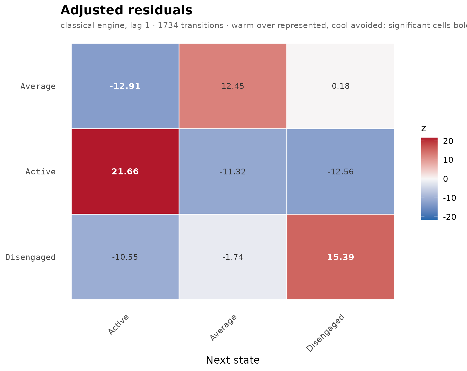

plot(fit, type = "network")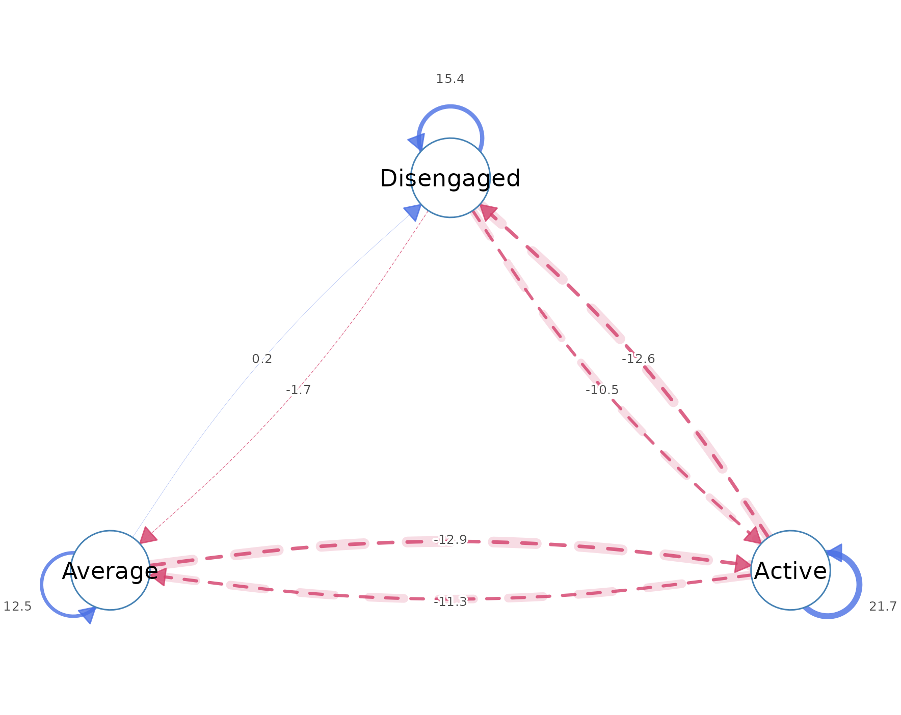

plot(fit, type = "network", weights = "tna")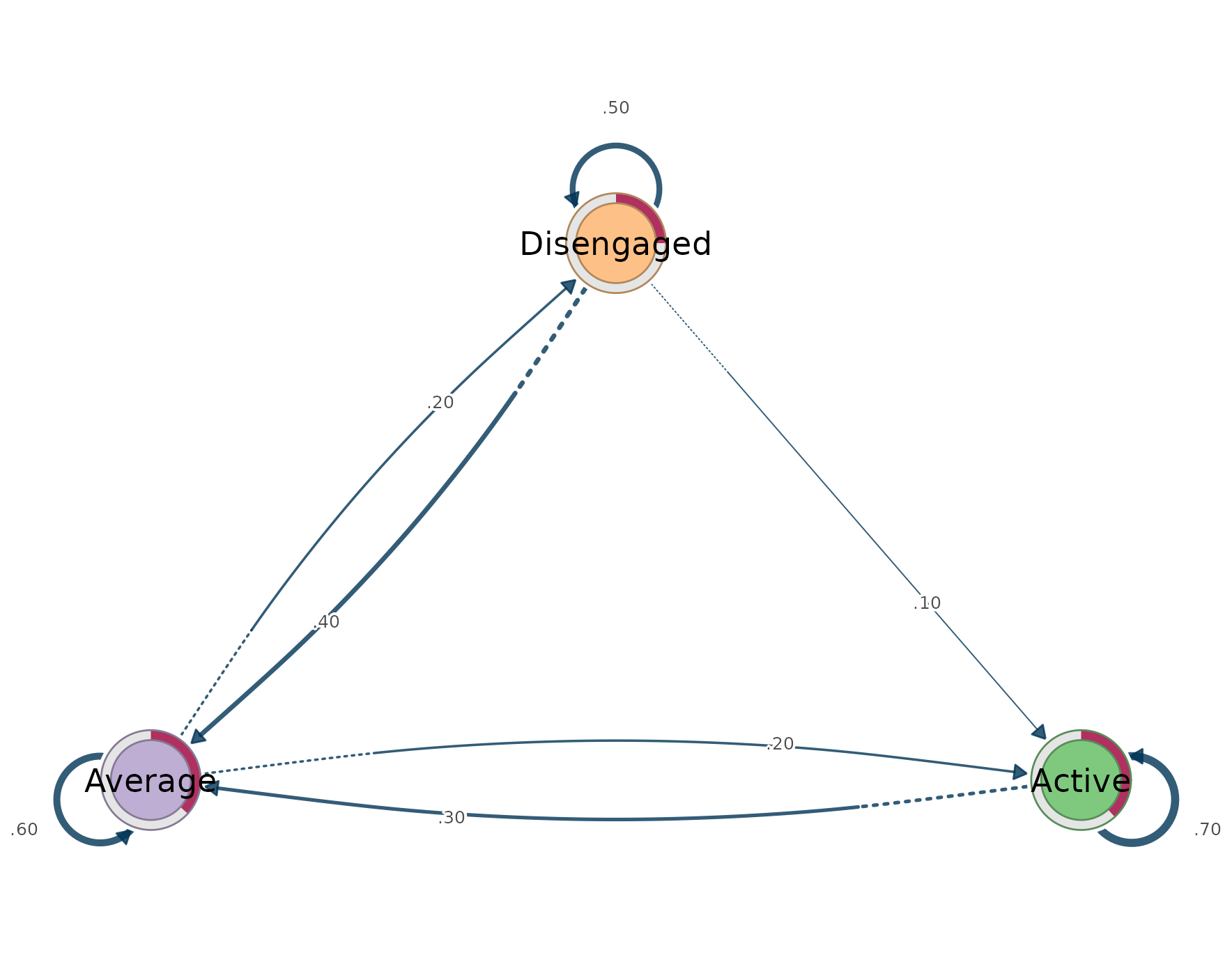

plot(fit, type = "chord")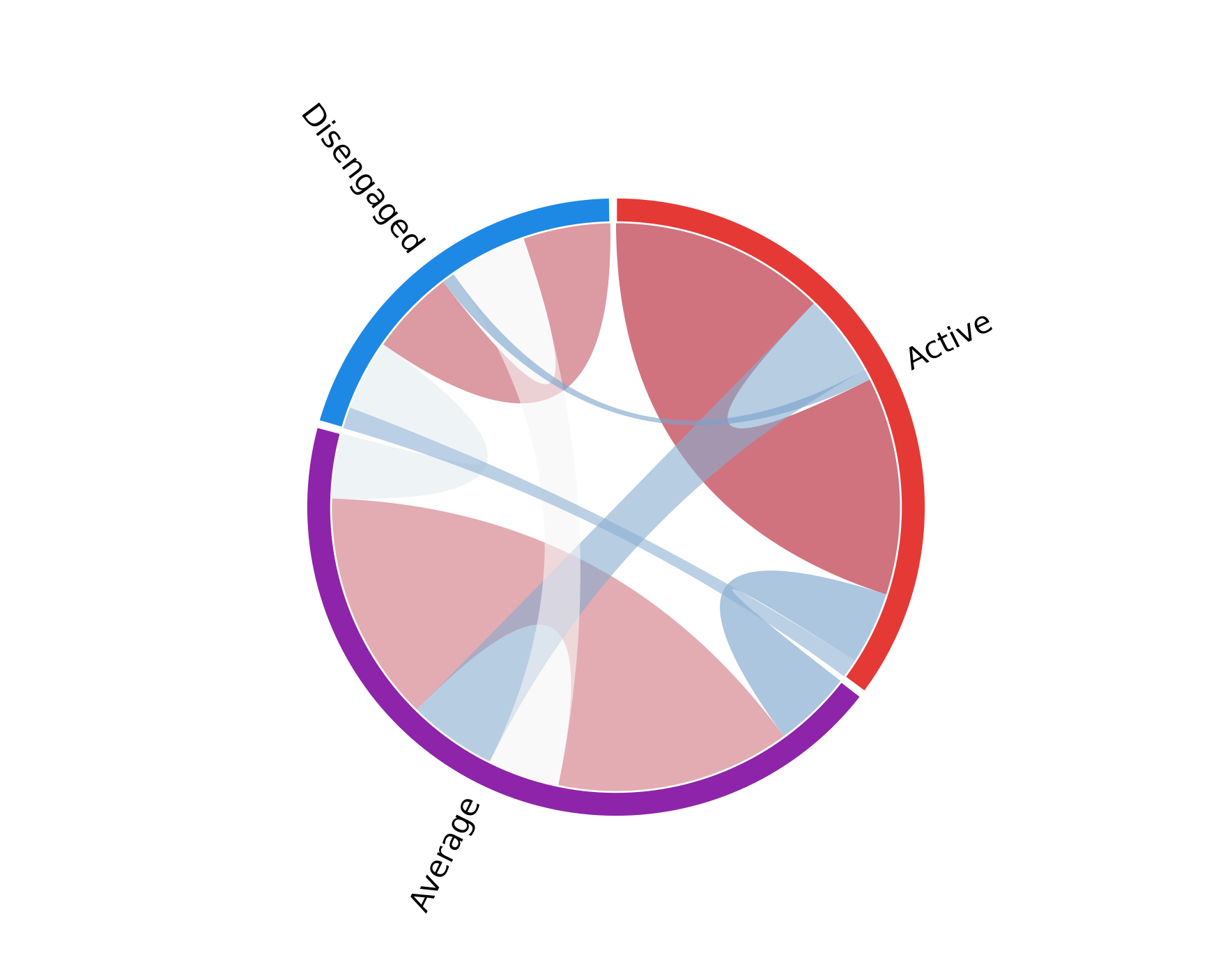

plot(fit, type = "sunburst")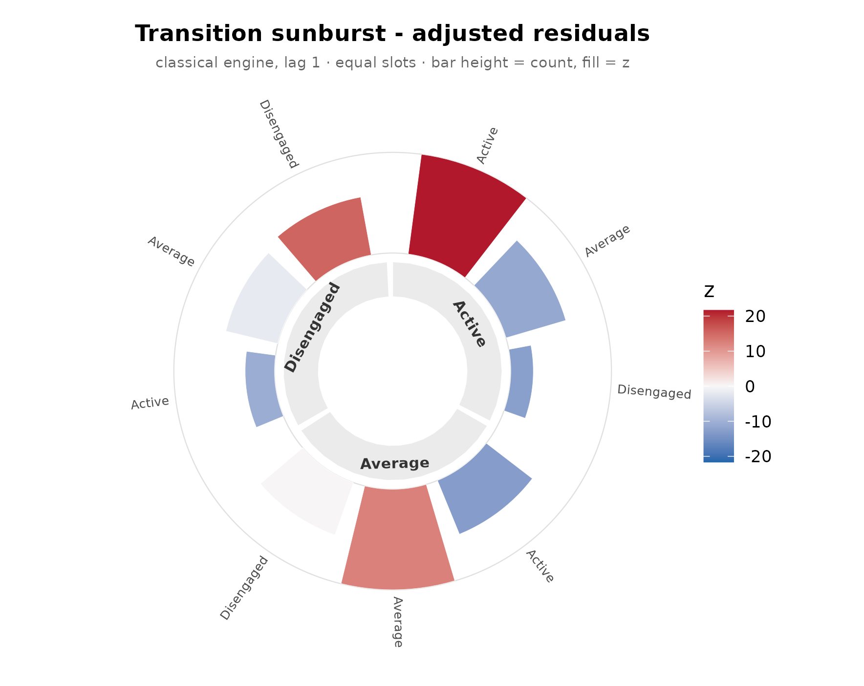

The full gallery, including the which = matrix selector and the grouped-plot variants, is in vignette("plotting", package = "lagdynamics").

Group comparison

A grouping variable produces one fit per group in a shared state space. Here the long-format group_regulation_long event log is split by achievement level, using the actor / action / time grammar.

gfit <- lsa(group_regulation_long, actor = "Actor", action = "Action",
            time = "Time", group = "Achiever")
gfit
#> <lsa_group>
#>   engine:    classical
#>   states:    9 (adapt, cohesion, consensus, coregulate, discuss, emotion, monitor, plan, synthesis)
#>   groups:    2
#>     - High:        1000 sequences
#>     - Low:         1000 sequences
transitions(gfit, significant = TRUE) |> head(4)
#>   group       from    to lag count expected    prob prob_col adj_res        p
#> 1  High  consensus adapt   1    14     38.1 0.00413   0.0979   -4.59 4.45e-06
#> 2  High coregulate adapt   1    20     10.0 0.02237   0.1399    3.27 1.06e-03
#> 3  High    discuss adapt   1    48     22.5 0.02396   0.3357    5.88 4.00e-09
#> 4  High    emotion adapt   1     5     17.4 0.00323   0.0350   -3.19 1.40e-03
#>   yules_q   kappa kappa_z  kappa_p  lift  sign significant
#> 1  -0.544 -0.6606   -4.98 6.36e-07 0.367 under        TRUE
#> 2   0.371  0.0636    2.90 3.68e-03 1.990  over        TRUE
#> 3   0.466  0.1803    5.21 1.86e-07 2.132  over        TRUE
#> 4  -0.589 -0.7375   -3.46 5.48e-04 0.287 under        TRUE
summary(gfit)
#>   group    engine lag n_states n_sequences n_events n_transitions n_significant
#> 1  High classical   1        9        1000    13721         12721            66
#> 2   Low classical   1        9        1000    13812         12812            67
#>   alpha lrx2 lrx2_df lrx2_p   x2 x2_df x2_p
#> 1  0.05 6147      64      0 6807    64    0
#> 2  0.05 7715      64      0 9197    64    0

compare_lsa() tests whether the groups differ, edge by edge, by permuting group labels over whole sequences – the unit that is actually exchangeable under the null – with optional multiplicity adjustment. bayes_compare_lsa() reaches the same question analytically, reporting the credible range of each group difference in transition probability. With more than two groups, both return pairwise results.

cmp <- compare_lsa(gfit, R = 100, adjust = "BH")
cmp
#> <lsa_comparison>
#>   groups:   High vs Low
#>   measure:  log_or difference (High - Low)
#>   R:        100 label permutations
#>   edges:    38 significant of 78 tested (adjust = BH)
#>   omnibus:  statistic = 79.48, p = 0.009901
transitions(cmp) |> head(4)
#>         from    to log_or_a log_or_b  diff p_perm  p_adj significant
#> 1      adapt adapt   -1.183    -3.17 1.984     NA     NA       FALSE
#> 2   cohesion adapt   -0.794    -3.92 3.127 0.0099 0.0234        TRUE
#> 3  consensus adapt   -1.219    -1.97 0.748 0.0693 0.1126       FALSE
#> 4 coregulate adapt    0.778    -1.08 1.855 0.0099 0.0234        TRUE

bcmp <- bayes_compare_lsa(gfit, draws = 1000, adjust = "BH", seed = 1)
bcmp
#> <lsa_bayes>  (Bayesian Dirichlet-Multinomial comparison)
#>   groups:    High vs Low
#>   prior:     Dirichlet(0.50)  |  draws: 1000  |  CI: 95%
#>   edges:     39 credibly different of 81 compared
transitions(bcmp) |> head(4)
#>         from    to  prob_a   prob_b     diff    ci_low ci_high    pd
#> 1      adapt adapt 0.00344 0.001342  0.00209 -0.005313 0.01663 0.650
#> 2   cohesion adapt 0.00584 0.000657  0.00518  0.001209 0.01097 0.989
#> 3  consensus adapt 0.00427 0.005609 -0.00134 -0.004714 0.00214 0.777
#> 4 coregulate adapt 0.02282 0.011569  0.01125  0.000315 0.02310 0.977
#>   effect_size p_value  p_adj significant
#> 1        0.39   0.700 0.8239       FALSE
#> 2        2.06   0.022 0.0435       FALSE
#> 3       -0.75   0.446 0.6123       FALSE
#> 4        1.91   0.046 0.0867       FALSE

plot(cmp)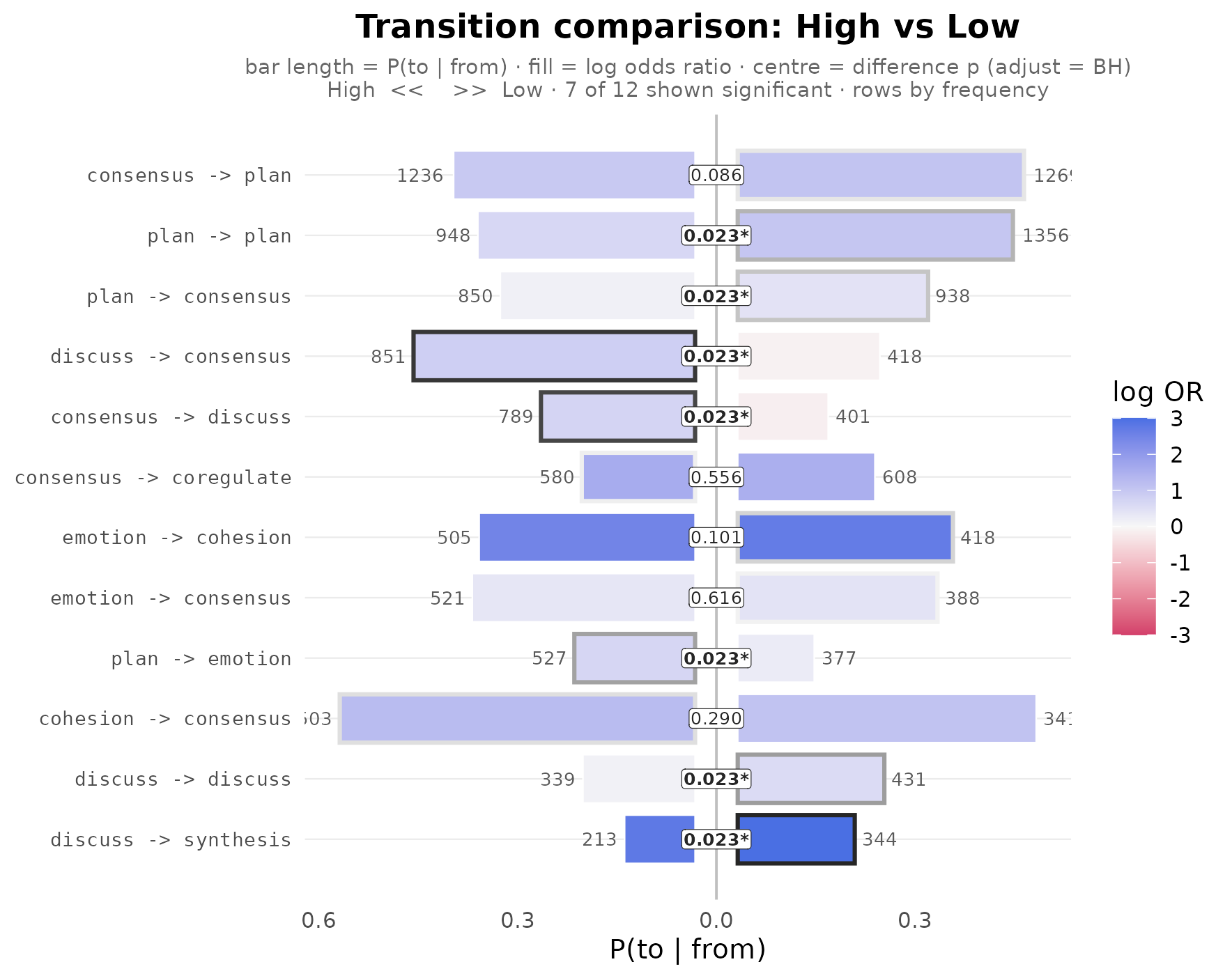

plot(cmp, style = "heatmap")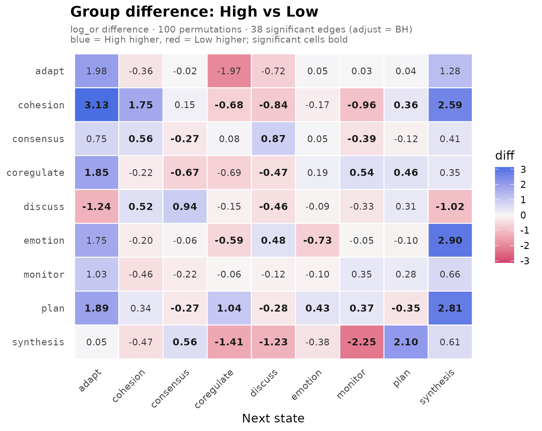

Confirmatory battery

The adjusted residual tests each edge against independence, but that test rests on large-sample assumptions that sequential data can violate, and stronger claims – about precision, robustness, or the network as a whole – need their own evidence. The battery pairs each kind of claim with a matching procedure:

claim	evidence	verb
a specific transition is real; how precise	edge-level uncertainty	`certainty_lsa()`, `bootstrap_lsa()`
a significant transition is not fragile	robustness to case loss	`stability_lsa()`
the whole network is reproducible	split-half reliability	`reliability_lsa()`
the structure exceeds chance	assumption-free empirical null	`permute_lsa()`
two groups differ	inference under exchangeability	`compare_lsa()`, `bayes_compare_lsa()`

cert <- certainty_lsa(fit)
transitions(cert) |> head(3)
#>         from     to observed prob_observed prob_mean prob_se prob_ci_low
#> 1     Active Active      459         0.698     0.697  0.0179      0.6611
#> 2    Average Active      153         0.204     0.204  0.0147      0.1760
#> 3 Disengaged Active       39         0.120     0.121  0.0180      0.0879
#>   prob_ci_high  p_value stable adj_res_observed adj_res_stable
#> 1        0.731 5.56e-20   TRUE             21.7           TRUE
#> 2        0.233 6.06e-04   TRUE            -12.9           TRUE
#> 3        0.158 9.45e-02  FALSE            -10.5          FALSE

boot <- bootstrap_lsa(fit, R = 50)
transitions(boot) |> head(3)
#>         from     to observed count_mean count_se count_ci_low count_ci_high
#> 1     Active Active      459      467.5    60.53          360           559
#> 2    Average Active      153      156.5    14.79          131           178
#> 3 Disengaged Active       39       38.7     5.46           28            49
#>   adj_res_observed adj_res_mean adj_res_se adj_res_ci_low adj_res_ci_high
#> 1             21.7         21.5       1.56           18.9           24.33
#> 2            -12.9        -12.8       1.44          -15.2          -10.20
#> 3            -10.5        -10.6       1.26          -12.7           -8.29
#>   adj_res_p_boot adj_res_stable prob_observed prob_mean prob_ci_low
#> 1              0           TRUE         0.698     0.696      0.6318
#> 2              0           TRUE         0.204     0.209      0.1729
#> 3              0           TRUE         0.120     0.121      0.0838
#>   prob_ci_high yules_q_observed yules_q_mean yules_q_ci_low yules_q_ci_high
#> 1        0.745            0.828        0.821          0.769           0.874
#> 2        0.250           -0.601       -0.593         -0.685          -0.493
#> 3        0.156           -0.698       -0.698         -0.802          -0.584

rel <- reliability_lsa(fit, R = 20)
rel
#> <lsa_reliability>
#>   engine:        classical
#>   replicates:    20
#>   weights:       prob
#>   method:        pearson
#>   n sequences:   136
#>   split-half r:  0.972  (sd = 0.025)
#>   95% CI:        [0.921, 0.996]

stab <- stability_lsa(fit, R = 30)
stab
#> <lsa_stability>
#>   engine:        classical
#>   replicates:    30
#>   proportion:    80%
#>   min stable:    95%
#>   stable edges:  7 of 9 (>= 95% across replicates)

pm <- permute_lsa(fit, R = 100)
pm
#> <lsa_permutation>
#>   engine:        classical
#>   replicates:    100
#>   within seq:    TRUE
#>   significant edges (p_perm < 0.050): 7 of 9

plot(boot)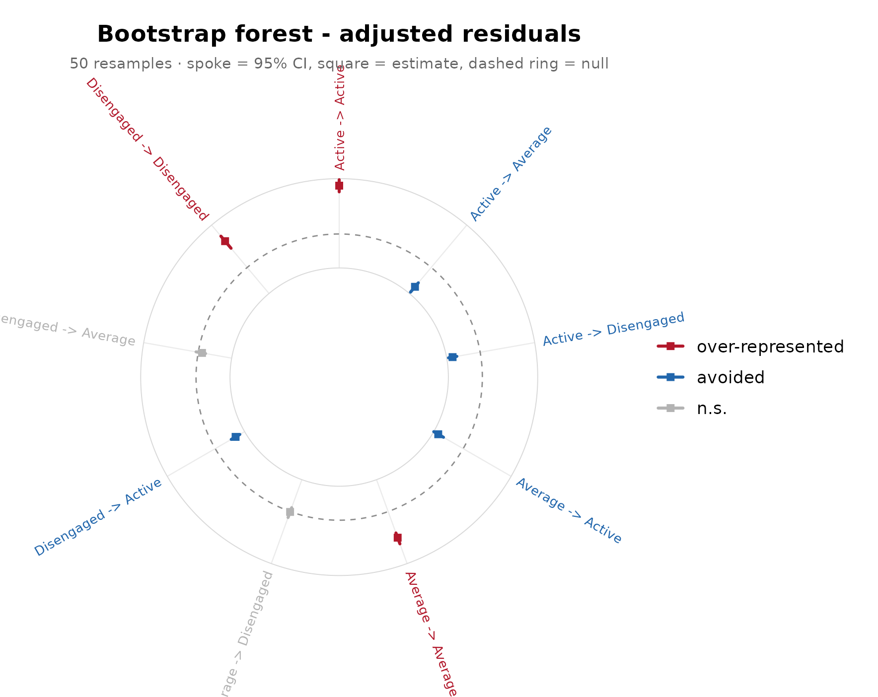

Bootstrap replication is reproducible across languages and sessions: bootstrap_lsa(indices = ) accepts a precomputed resampling matrix for bit-identical replay. The full treatment of the battery is in vignette("confirmatory", package = "lagdynamics").

Interoperability

lagdynamics is designed to sit inside an existing analysis stack rather than replace it, on both the input and the output side.

Input. lsa() accepts, through one front door:

wide data frames and matrices (rows = sequences, columns = ordered positions), as in the bundled engagement and group_regulation;
lists of categorical vectors, one element per sequence;
long event logs via the actor / action / time grammar, including Unix and custom time formats, as in group_regulation_long and ai_long;
foreign sequence objects, duck-typed so that none of their packages becomes a runtime dependency: TraMineR state sequences (stslist), tna models and their grouped and sequence-data forms (tna, group_tna, tna_seq_data, tna_data), and Nestimate prepared data (nestimate_data).

fit_log <- lsa(group_regulation_long, actor = "Actor",
               action = "Action", time = "Time")
fit_log
#> Lag Sequential Analysis  -  classical  (lag 1, directed)
#>   9 states | 25533 transitions | 27533 events | 2000 sequences
#>   states: adapt, cohesion, consensus, coregulate, discuss, emotion, monitor, plan, synthesis
#>   independence: G² = 13203.8, df = 64, p <2e-16
#> 
#>   Significant transitions (p < 0.05): 72 of 81
#>   strongest over-represented (of 23):
#>     emotion -> cohesion      z =  +58.2  ***
#>     discuss -> synthesis     z =  +48.0  ***
#>     synthesis -> adapt       z =  +38.8  ***
#>     consensus -> coregulate  z =  +35.3  ***
#>     consensus -> plan        z =  +32.6  ***
#>     ... and 18 more
#> 
#>   Initial states:
#>     consensus  0.214  ████████████████████████
#>     plan       0.204  ███████████████████████
#>     discuss    0.175  ████████████████████
#>     emotion    0.151  █████████████████
#>     monitor    0.144  ████████████████
#>     cohesion   0.060  ███████
#>     synthesis  0.019  ██
#>     coregulate 0.019  ██
#>     adapt      0.011  █

Output. The fitted object carries its network identity with it: it inherits the cograph_network class, so cograph’s rendering verbs accept it directly, and the plotting gallery above draws its network, chord, and comparison views through that seam. The fitted probabilities are exposed for any downstream transition-network tooling – transition_probabilities() returns the row-stochastic matrix $P(\text{to} \mid \text{from})$ and initial() the initial-state distribution, the two ingredients a TNA-style model requires – and every result object reads as a plain data frame through transitions(), so results move into any tabular pipeline without package-specific code.

transition_probabilities(fit)
#>            Active Average Disengaged
#> Active      0.698   0.267      0.035
#> Average     0.204   0.610      0.186
#> Disengaged  0.120   0.397      0.483
initial(fit)
#>        state init_prob
#> 1     Active     0.382
#> 2    Average     0.368
#> 3 Disengaged     0.250

Bundled data

Four data sets ship with the package, spanning the supported input shapes: engagement (wide; 138 students, weekly engagement states), group_regulation (wide; 2,000 collaborative-learning sessions), group_regulation_long (long event log with actor, action, time, and an achievement group), and ai_long (long event log of coded AI actions in human–AI coding sessions).

Mohammed Saqr

Sonsoles López-Pernas