Circular Bootstrap Forest of an LSA Fit

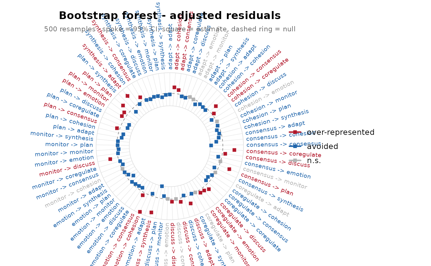
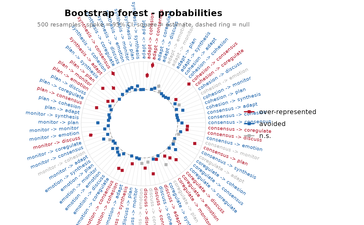
Draws a radial forest of an bootstrap_lsa() result: each transition is a spoke around a ring, spanning its bootstrap confidence interval, with a square at the observed estimate and a dashed reference ring at the null. Spokes whose adjusted residual is significant across resamples are coloured by direction (warm = over-represented, cool = avoided); non-significant ones are grey. Needs ggplot2.

Usage

plot_forest(
  boot,
  metric = c("residuals", "count", "prob", "yules_q"),
  n_top = NULL,
  show_nonsig = TRUE,
  label_size = 2.6
)

# S3 method for class 'lsa_bootstrap'
plot(x, ...)

Arguments

boot

An lsa_bootstrap object from bootstrap_lsa().

metric

Which bootstrapped quantity to plot: "residuals" (default, adjusted residual), "count", "prob", or "yules_q".

n_top

Optional integer: keep only the n_top edges with the largest absolute estimate (the rest are dropped). Default NULL (all edges).

show_nonsig

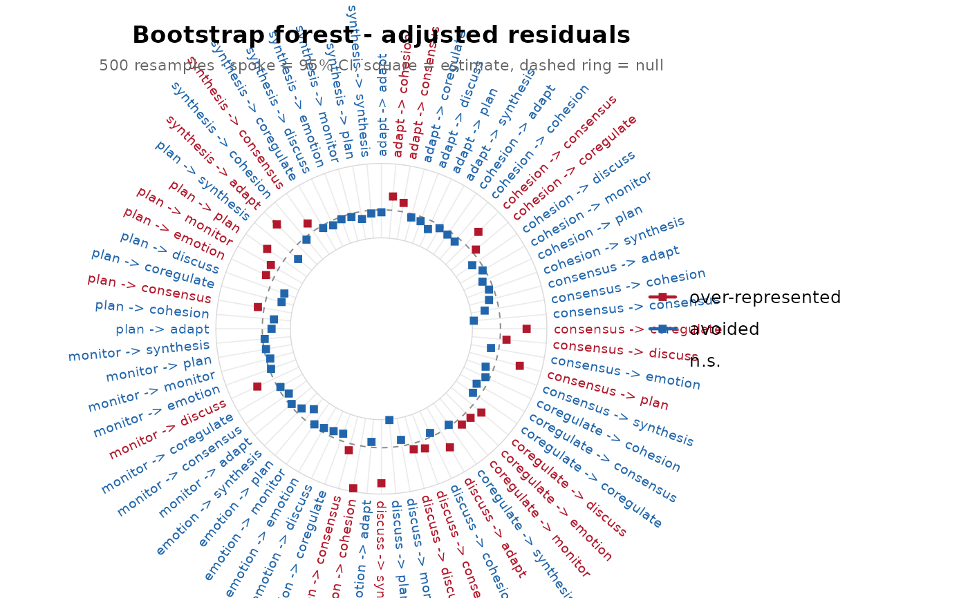
Logical. Draw non-significant edges (grey). Default TRUE; set FALSE to keep only significant transitions.

label_size

Edge-label text size. Default 2.6.

x

An lsa_bootstrap object (for the plot() method).

...

Passed to plot_forest() (e.g. metric, n_top).

Value

A ggplot object (drawn when printed).

See also

bootstrap_lsa(), plot.lsa() (heatmap), plot_polar() (sunburst)

Examples

# \donttest{
fit <- lsa(group_regulation)
b <- bootstrap_lsa(fit, R = 500)
plot_forest(b)                       # residual CIs, circular

plot_forest(b, metric = "prob")      # probability CIs

plot_forest(b, show_nonsig = FALSE)  # significant transitions only

# }