Polar Sunburst of an LSA Fit

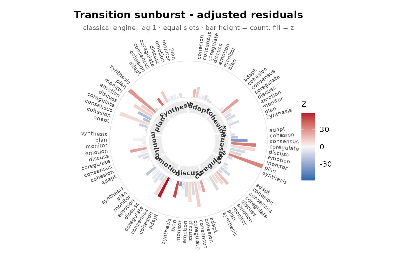
Draws the transition structure as a polar sunburst with the source states named along a large inner ring. Two styles: "rose" (default) gives every target an equal angular slot and encodes frequency as the radial bar height (so nothing crams); "wedge" sizes each transition's angular width by its frequency share (the classic look), omitting tiny wedges. Both fill by the adjusted residual (warm = over-represented, cool = avoided), sharing the plot.lsa() heatmap colour scale. Needs ggplot2.

Usage

plot_polar(
  fit,
  style = c("rose", "wedge"),
  fill = c("residuals", "prob", "lift"),
  size = c("count", "prob"),
  significant = FALSE,
  labels = c("all", "auto", "none"),
  min_show = 0.01,
  label_size = 3,
  ...
)

Arguments

fit: An lsa fit from lsa().
style: "rose" (default, equal slots + bar height) or "wedge" (frequency-proportional wedge width).
fill: Which quantity fills the bars/wedges: "residuals" (default, diverging), "prob", or "lift".
size: For style = "rose", which non-negative quantity sets bar height: "count" (default) or "prob". Ignored for "wedge".
significant: Logical. Grey out non-significant cells (keeping their size). Default FALSE.
labels: Which target cells to name: "all", "auto", or "none". Default is "all" for "rose" (equal slots leave room) and "auto" for "wedge" (only wedges wide enough to fit a name). Source names are always shown.
min_show: For style = "wedge", drop wedges whose frequency share of their source's outflow is below this fraction. Default 0.01; 0 keeps all.
label_size: Label text size. Default 3.
...: Ignored; accepted so plot(fit, type = "sunburst", ...) can forward arguments without error.

Value

A ggplot object (drawn when printed).

Examples

fit <- lsa(group_regulation)
plot_polar(fit)                          # rose: bars filled by residual

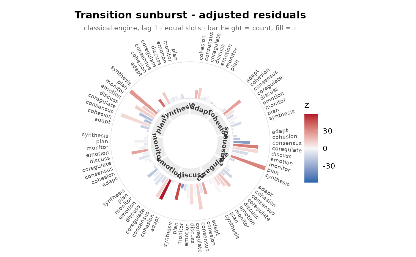plot_polar(fit, style = "wedge")         # classic frequency wedges

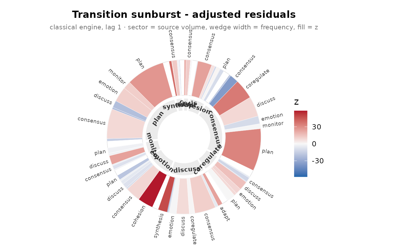plot_polar(fit, significant = TRUE)      # non-significant cells greyed

Usage

Arguments

Value

See also

Examples