An idiographic model is estimated from the observations of a single person, so the quality of that person’s data limits what the model can show. Before any model is fitted, descriptive statistics are therefore computed separately for each person and each variable. These are the number of observations and missing values, the spacing of the occasions, the mean and the range, the standard deviation, the change from one occasion to the next, and the correlation of each occasion with the previous one. These statistics establish whether the data of each person can be analysed and reveal the problems that would distort the results.
The first problem is a short series. Every coefficient of a person’s model is estimated from that person’s observations alone, and a series with few observations gives unstable estimates and supports only a small model. Missing occasions and long gaps between occasions shorten the series further and break the regular spacing that lagged effects assume, because a lag that spans one day for one pair of observations and a week for another mixes two different quantities.
The second problem is low variability. A variable that changes little within a person carries little information about its effects, and its coefficient has a wide confidence interval. A variable that is constant within a person cannot be estimated as a predictor at all. Responses gathered at the floor or ceiling of the scale restrict the range in the same way and weaken the observed associations.
The third problem is dependence over time. A series with a trend changes level over the study period, and two variables that both trend appear related even when their daily fluctuations are unrelated. A series with strong autocorrelation carries each day’s value into the next day, so its observations are less informative than their number suggests. Long runs of identical responses can indicate careless responding.
The fourth problem concerns the level of the variation. Part of the variance of a variable lies between persons, in their means, and part lies within persons, in their daily fluctuations. A correlation computed across all observations mixes the two parts, and the share of each determines whether the variable is suited to a within-person analysis.
Data
The examples use 12 learners from srl, a data frame in
long format with one row per learner and day. Each learner rated
self-efficacy, effort and seven other indicators of self-regulated
learning once a day for 156 days.
Level and variability
Level and variability are the basic properties of a time series. The level is the typical value of a person’s responses, given by the mean and the median. The variability is the amount by which the responses change over time, and it determines how much the series can show about the effects of its variable. A variable that stays at nearly the same value for 156 days shows little of what happens when it changes.
The variability of each series is measured in two ways. The standard deviation (SD) measures the spread of a person’s observations around that person’s mean over the whole study. The root mean square successive difference (RMSSD) measures the size of the change from one occasion to the next. A series that drifts slowly over a wide range and a series that alternates sharply from day to day can have the same SD, and the second has the larger RMSSD (Jahng et al. 2008). The two are linked by the lag-1 autocorrelation , the correlation of each occasion with the previous one. For a stationary series , so the RMSSD is about 1.41 times the SD when consecutive days are unrelated, and smaller when each day carries over into the next.
describe_persons() returns one row per person and
variable, with the number of observations, the missing values, the span
of the occasions and the gaps between them, the level and the
variability. The argument time orders the observations, and
the successive differences and the autocorrelation are computed in that
order.
describe_persons(analysis_data, id = "name", vars = c("efficacy", "effort"),
                 time = "day", subject = c("Aisha", "Alice"))
#> PERSON DESCRIPTIVES
#>   Grouping    name
#>   Time        day
#>   People      2
#>   Variables   2
#>
#>   subject   variable     n   miss     mean   median       sd     min       max    rmssd   autocor      span   gap_median   gap_max
#> ----------------------------------------------------------------------------------------------------------------------------------
#>   Aisha     efficacy   156      0   56.919   61.765   21.034   0.000   100.000   26.881     0.169   155.000        1.000     1.000
#>   Alice     efficacy   156      0   35.761   36.364   20.614   0.000   100.000   28.790     0.024   155.000        1.000     1.000
#>   Aisha     effort     156      0   77.646   82.540   18.080   0.000   100.000   23.724     0.132   155.000        1.000     1.000
#>   Alice     effort     156      0   59.875   60.811   21.108   0.000   100.000   30.319    -0.032   155.000        1.000     1.000
#>
#>   sd    = overall spread;  rmssd = occasion-to-occasion change
#>   autocor = lag-1 carry-over (inertia)
Aisha and Alice each have 156 observations and no missing values. Their mean efficacy is 57 and 36, both have an SD of 21, and their RMSSDs are 27 and 29. The two learners differ in their typical level of efficacy and have similar day-to-day variability.
The figure plots the SD against the RMSSD for the 12 learners, with one point per learner and variable.
descriptives <- describe_persons(analysis_data, id = "name",
                                 vars = c("efficacy", "effort"), time = "day")
plot_descriptives(descriptives)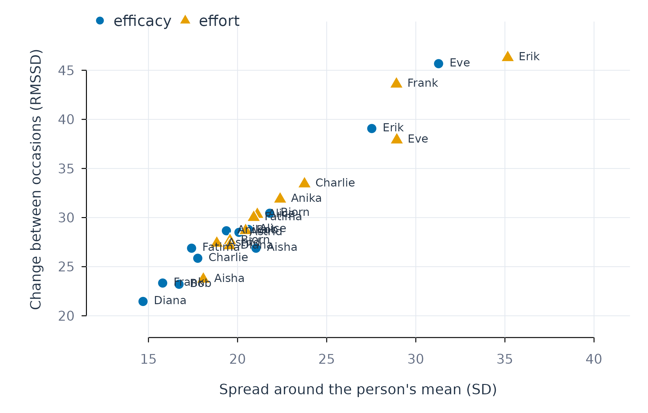
Figure 1. Spread (SD) against day-to-day change (RMSSD) for efficacy and effort in 12 learners.
The RMSSD lies between 1.28 and 1.54 times the SD, close to the value of 1.41 for unrelated consecutive days, so the learners carry little over from one day to the next. Erik and Eve have the largest spread and the largest daily change in both efficacy and effort. Diana, Frank and Bob vary least in efficacy, and Frank’s effort is among the most variable, so a learner can be stable on one variable and variable on another.
With detail = "full", the table adds the proportions of
responses at the floor and ceiling of the scale, the skewness and
kurtosis, the probability of an acute change between consecutive
occasions, the linear trend over the study and the longest run of
identical responses. These columns detect the restricted range, the
trends and the careless responding described above. Missing occasions
reduce the number of consecutive pairs from which the RMSSD and the
autocorrelation are computed.
Within-person correlations
A within-person correlation quantifies the covariation of two variables across the occasions of one person. It indicates which states co-occur within an individual, and its sign and magnitude differ between individuals. A correlation computed over the pooled observations of a sample combines within-person and between-person covariation, and it can differ from the within-person correlation of every individual in the sample. In the pooled observations of the 12 learners, monitoring and effort correlate at 0.10. The within-person correlations of the same pair range from −0.47 to 0.52 and are negative for 3 of the 12 learners.
The within-person correlation is the Pearson correlation of two
variables computed from the observations of one person. A positive
correlation indicates that on occasions when one variable exceeds the
person’s mean, the other variable also tends to exceed its mean.
correlate_persons() returns one row per person and pair of
variables, with the correlation, the number of complete pairs and a 95%
confidence interval based on Fisher’s
transformation.
correlations <- correlate_persons(analysis_data, id = "name",
                                  vars = c("efficacy", "monitoring", "effort"),
                                  time = "day", subject = c("Aisha", "Alice"))
correlations
#> PERSON-SPECIFIC CORRELATIONS
#>   Grouping   name
#>   People     2
#>   Pairs      3
#>
#>   subject   x            y              n        r           95% CI          p
#> ------------------------------------------------------------------------------
#>   Aisha     efficacy     monitoring   156    0.394     [0.25, 0.52]    < 1e-04
#>   Aisha     efficacy     effort       156    0.352     [0.21, 0.48]    < 1e-04
#>   Aisha     monitoring   effort       156    0.284     [0.13, 0.42]   0.000325
#>   Alice     efficacy     monitoring   156   -0.231   [-0.37, -0.08]   0.003736
#>   Alice     efficacy     effort       156    0.491     [0.36, 0.60]    < 1e-04
#>   Alice     monitoring   effort       156   -0.352   [-0.48, -0.21]    < 1e-04
For Aisha, all three pairs are positively correlated, with coefficients between 0.28 and 0.39. For Alice, efficacy and effort are positively correlated (r = 0.49), and monitoring is negatively correlated with efficacy (r = −0.23) and with effort (r = −0.35). Alice reports lower effort and lower efficacy on occasions of higher monitoring.
The figure plots each correlation with its 95% confidence interval, ordered by magnitude.
plot_correlations(correlations)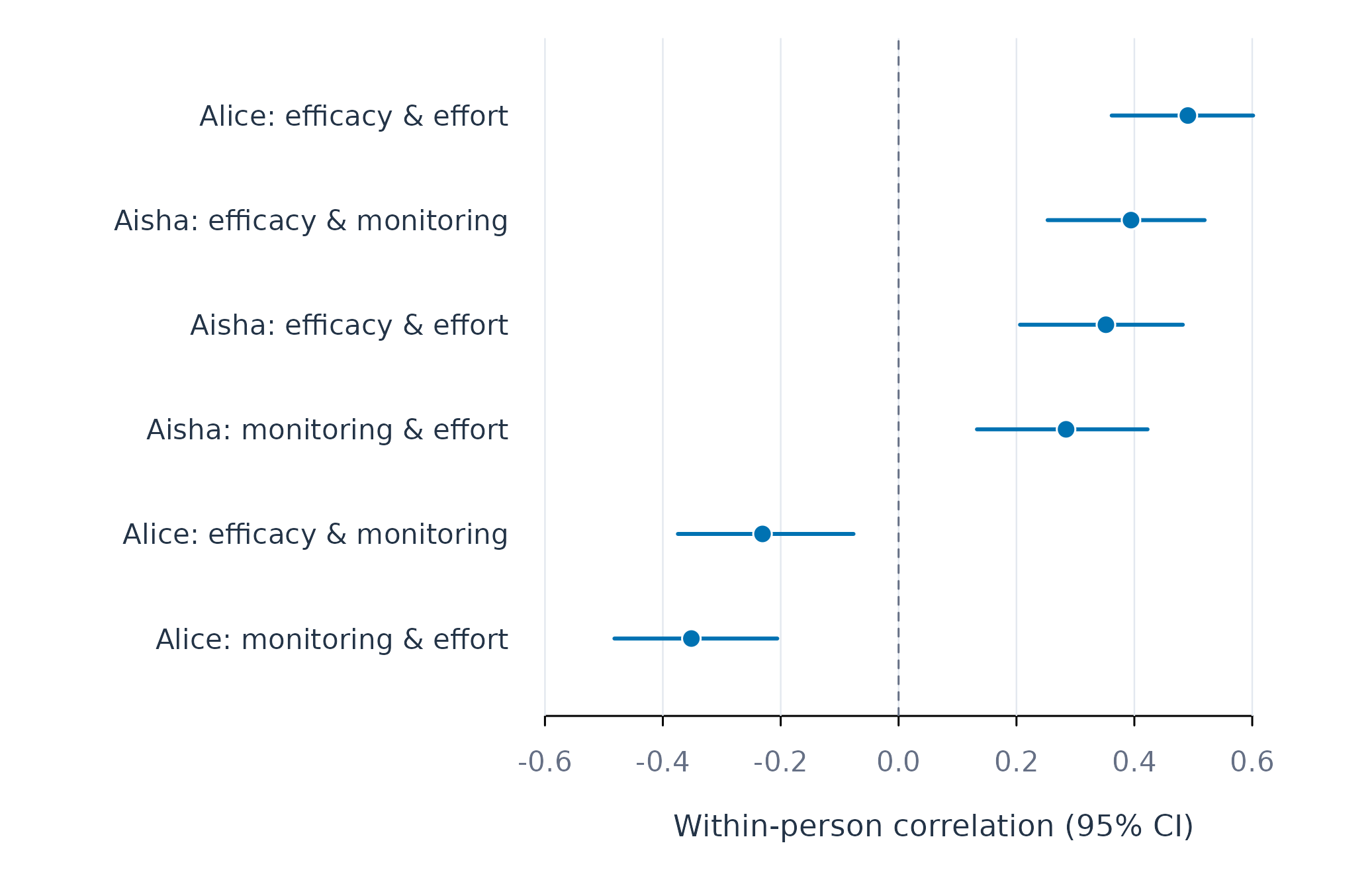
Figure 2. Within-person correlations with 95% confidence intervals for two learners.
Of the 6 intervals, 6 lie entirely on one side of zero.
The coefficients describe concurrent associations, measured on the
same occasion, and each is a bivariate association unadjusted for the
remaining variables. Temporal precedence is examined with lagged
regressions and dynamic networks. Serial dependence between consecutive
daily observations makes the confidence intervals too narrow when the
autocorrelation is strong. The argument min_n sets the
minimum number of complete pairs for a coefficient to be reported, and a
variable that is constant within a person yields a missing
coefficient.
Between-person and within-person variance
Person-specific models use only the fluctuation of each person around that person’s mean. Analyses that combine persons, such as pooled regressions, multilevel models and the comparison of individual with pooled estimates, use both the differences between person means and the fluctuation within persons. For these analyses, the partition of the variance determines how each variable enters the model. Between-person variance arises from differences in the person means, and within-person variance arises from the fluctuation of each person around that person’s mean.
The intraclass correlation (ICC) is the between-person share of the
total variance. A large ICC indicates that much of the variance reflects
stable differences between persons. An association computed on the raw
scores of all persons is then largely an association between person
means. Such a variable enters a pooled analysis as a person mean and a
deviation from it, so that the within-person and between-person effects
are estimated separately with split_levels() and
fit_within_between(). The ICC is a property of the sample,
computed over all persons. The within-person variability of an
individual is assessed with the SD and RMSSD of that individual’s
series. The reliability of the person means indicates how precisely the
between-person part of a variable is measured, and an unreliable person
mean biases the between-person and contextual effects.
components <- variance_components(analysis_data, id = "name",
                                  vars = c("efficacy", "monitoring", "effort"))
components
#> VARIANCE COMPONENTS
#>   Grouping   name
#>   Method     anova
#>
#>                  Within    Between     ICC   Reliability
#> --------------------------------------------------------
#>   efficacy     435.4422   290.6398   0.400         0.990
#>   monitoring   516.7891   313.4551   0.378         0.990
#>   effort       560.3849   194.4532   0.258         0.982
#>
#>   ICC         share of variance lying BETWEEN groups
#>   Reliability precision of each group's own mean
The ICCs are 0.40 for efficacy, 0.38 for monitoring and 0.26 for effort, so between 60% and 74% of the variance of each variable lies within learners, the part that person-specific models use. The between-person share is substantial for all three variables, and in a pooled analysis each is decomposed into a person mean and a deviation before entering the model. The reliability of the person means exceeds 0.98 for all three variables, because each mean is computed from about 156 observations.
The figure plots the between-person and within-person share of the variance of each variable.
plot_variance(components)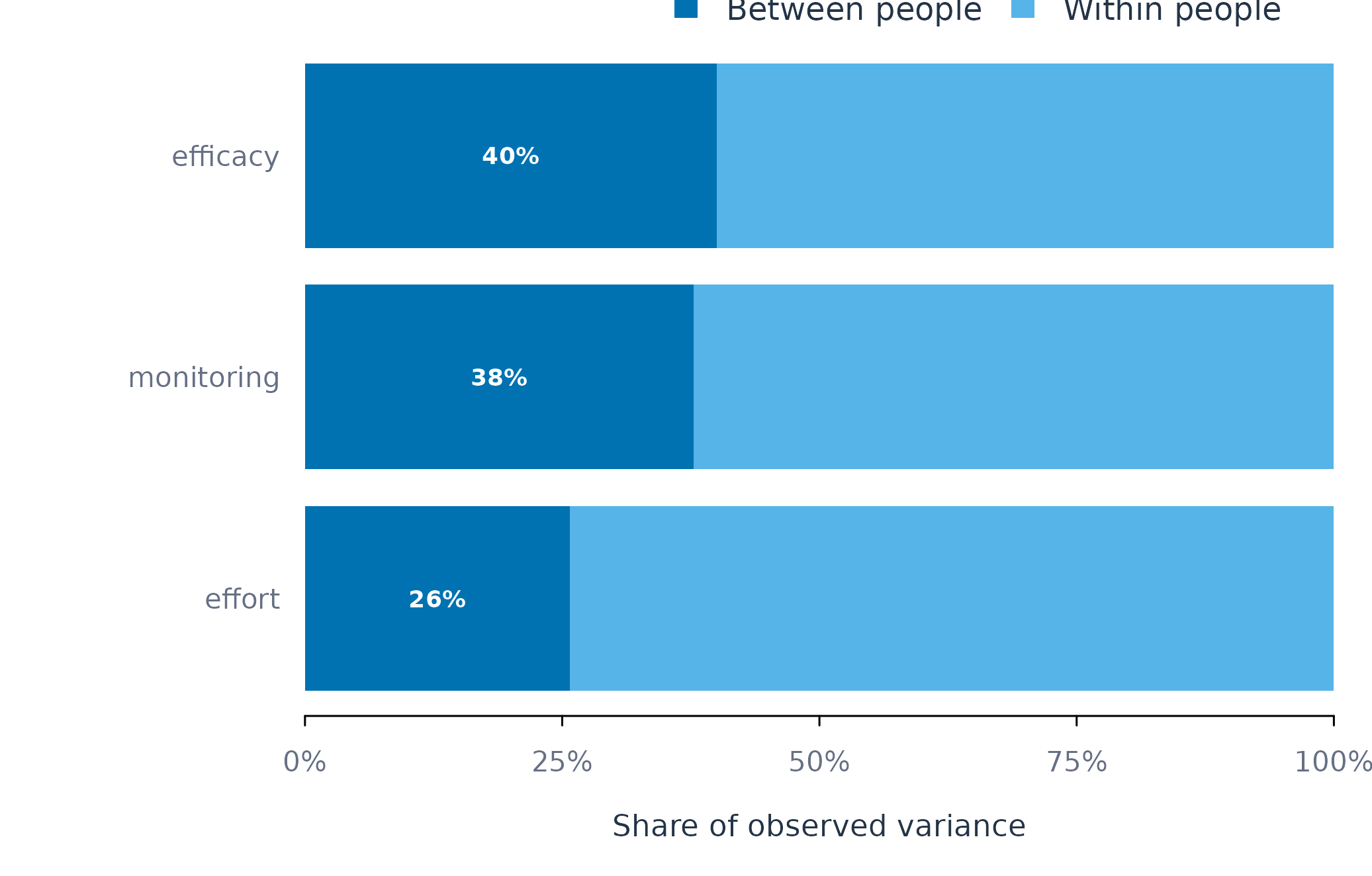
Figure 3. Between-person and within-person shares of variance.
A variable that is constant within persons supports only between-person comparisons, and a variable without between-person variance supports only within-person analysis.
Within-person and between-person correlations
Findings obtained from a group are often taken to describe the individuals in that group. The inference from the group to the individual holds when the process is ergodic, that is, when the relations among the variables are the same within every person and stable over time (Molenaar 2004). Fisher, Medaglia and Jeronimus (2018) proposed a direct test of this generalisation for correlations. For one pair of variables, two distributions of correlations are compared. The within-person distribution contains one correlation per person, computed across that person’s occasions. The between-person distribution contains one correlation per occasion, computed across persons. The first observations of all persons form one cross-sectional sample, the second observations form a second one, and so on. When group-level results generalise to individuals, the two distributions have similar means and similar spreads. Across six samples, Fisher and colleagues found the within-person standard deviation to be two to four times the between-person standard deviation.
The comparison uses all 36 learners in srl, so each
between-person correlation rests on 36 persons and each within-person
correlation on up to 156 occasions. correlate_levels()
returns one row per pair of variables, with the mean and standard
deviation of each distribution and the ratio of the two standard
deviations.
levels_result <- correlate_levels(srl, id = "name",
                                  vars = c("efficacy", "monitoring", "effort"),
                                  time = "day")
levels_result
#> WITHIN- VERSUS BETWEEN-PERSON CORRELATIONS
#>   Grouping       name
#>   Lag adjusted   no
#>
#>   x            y            persons   mean     SD   occasions   mean     SD   SD ratio
#> --------------------------------------------------------------------------------------
#>   efficacy     monitoring        36   0.27   0.30         156   0.29   0.14       2.11
#>   efficacy     effort            36   0.36   0.25         156   0.50   0.14       1.82
#>   monitoring   effort            36   0.25   0.32         156   0.28   0.14       2.30
#>
#>   within: one r per person;  between: one r per occasion
#>   SD ratio = within SD / between SD
For efficacy and monitoring, and for monitoring and effort, the mean correlations at the two levels are close (0.27 and 0.29; 0.25 and 0.28). For efficacy and effort, the mean within-person correlation (0.36) is lower than the mean between-person correlation (0.50). For all three pairs, the within-person correlations are more dispersed, with a standard deviation 1.82 to 2.30 times that of the between-person correlations. For two of the three pairs, the correlation across learners approximates the average within-learner correlation, and the correlations of the individual learners are distributed about twice as widely around it.
The figure plots the two distributions as density curves. The ticks below each curve mark the individual correlations, and the vertical lines mark the means.
plot_levels(levels_result)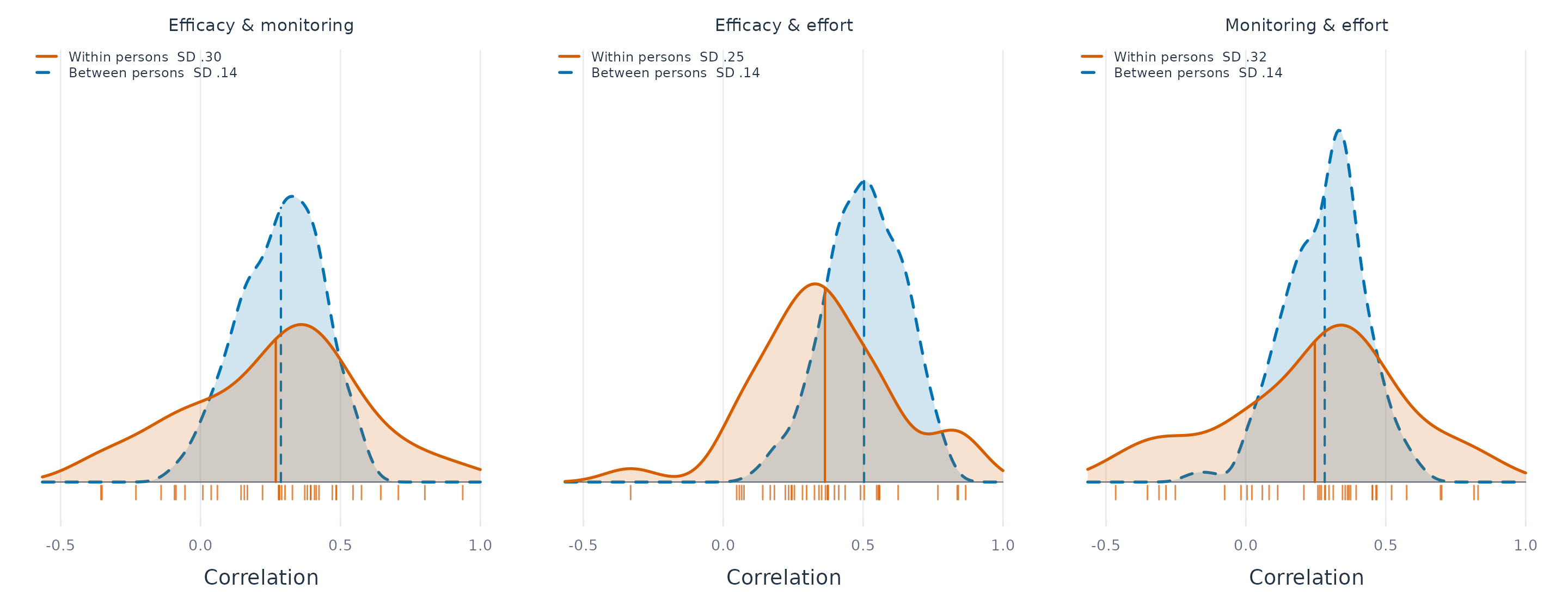
Figure 4. Distributions of within-person correlations (one per learner, solid) and between-person correlations (one per occasion, dashed) for three pairs of variables.
Serial dependence within persons can inflate the spread of the
within-person correlations. With lag_adjust = TRUE, each
variable is first regressed on its own lag-1 value and on the lag-1
value of the other variable, and the within-person correlations are
computed from the residuals.
lagged_levels <- correlate_levels(srl, id = "name",
                                  vars = c("efficacy", "monitoring", "effort"),
                                  time = "day", lag_adjust = TRUE)
summary(lagged_levels)
#>            x          y n_within mean_within median_within sd_within n_between
#> 1   efficacy monitoring       36   0.2710705     0.2988340 0.3057933       156
#> 2   efficacy     effort       36   0.3674765     0.3562763 0.2499535       156
#> 3 monitoring     effort       36   0.2450722     0.2813312 0.3205831       156
#>   mean_between median_between sd_between mean_difference sd_ratio
#> 1    0.2873413      0.2979134  0.1446419     -0.01627083 2.114140
#> 2    0.5034717      0.5096236  0.1373181     -0.13599523 1.820251
#> 3    0.2818936      0.3080957  0.1397777     -0.03682132 2.293521
The adjustment changes the mean within-person correlations by at most 0.004, and the ratios of the standard deviations remain between 1.82 and 2.29. The lag-1 autocorrelations in Figure 1 are small, and the larger spread of the within-person correlations reflects differences between learners in the covariation of the variables.
The between-person correlations require occasions that are comparable across persons, and here the -th observation of every learner is treated as one occasion. With few persons, each between-person correlation rests on a small sample, and its sampling error adds to the between-person spread. The ratio of the standard deviations is a descriptive index and is reported without a significance test.
From description to models
The descriptions identify the persons and variables that can be
analysed and the form in which the variables enter the models. Series
that are short, sparse or nearly constant are excluded or analysed with
fewer predictors. Variables with a substantial between-person share are
decomposed into person means and deviations. The within-person
correlations and their spread indicate how far a pooled estimate
describes the individual learners. The person-specific estimates are
then modelled and compared with the pooled estimate using
fit_lm(), fit_within_between() and
pool_coefs().