
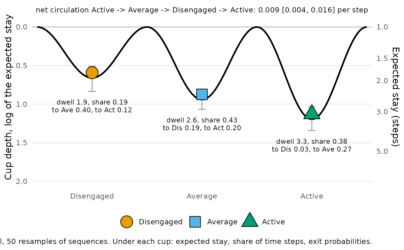
stability_landscape() estimates the ball-in-cup landscape (Scheffer et
al. 2009) of a transition network, which plot() draws: one cup per
state, whose depth is the stability of that state, how long the process
stays once it is there. A
state with stay probability \(P_{ii}\) is left after
\(1 / (1 - P_{ii})\) steps on average (its expected stay, or dwell
time), and its cup depth is the log of that time, \(-\log(1 - P_{ii})\),
so that dwell time = \(e^{depth}\): the escape-time law of a particle in
a potential well (Kramers 1940). A state that is left at once has depth 0,
no cup at all. It takes a "relative" or "frequency" network, a grouped
network (one landscape per group, on one state order) or the wide
sequences themselves, and gives every depth a percentile interval from
resampling whole sequences.
Depth is a property of the state alone. How often the process enters the
state is its share of the observed time steps, reported beside the
depth, and where the process goes when it leaves is in the exit
probabilities (summary(x, table = "exits")), which the plot writes under
each cup. With three states the result also reports the net circulation,
the net probability flux \(\pi_i P_{ij} - \pi_j P_{ji}\) around the
cycle, which stationarity makes equal on all three edges (Schnakenberg
1976): zero for a chain whose every transition is as common as its
reverse. The depths pool every sequence and every time step; whether they
change over the programme or along a covariate is what landscape_trend()
shows, and how long the process takes to get from one state to another is
given by passage_time().
Usage
stability_landscape(
  x,
  states = NULL,
  iter = 1000L,
  ci_level = 0.95,
  seed = NULL,
  cols = NULL
)

# S3 method for class 'net_landscape'
summary(object, table = c("cups", "exits", "circulation"), ...)

# S3 method for class 'net_landscape'
print(x, digits = 2, ...)

# S3 method for class 'net_landscape'
plot(x, ...)
Arguments
- x
The network or sequences: a transition network from
build_network()with method"relative"or"frequency"(or a barecograph_networkof one), a grouped one (netobject_group, for examplebuild_network()of abuild_clusters()result), atnamodel, or a wide sequence data frame or matrix. A network must carry its sequences; a network of another method (for example"glasso") raises an error of classnestimate_not_markov. For theprint()andplot()methods: anet_landscapeobject.- states
Every state, each named once, in the order to draw them (for example from least to most engaged). Default
NULL, the alphabetical order. A vector that leaves out, adds or repeats a state raises an error of classnestimate_bad_input.- iter
The number of bootstrap resamples of sequences behind the intervals, a non-negative whole number. Default
1000;0skips the resampling and leaves the intervalsNA.- ci_level
The interval level, a number between 0 and 1. Default
0.95.- seed
A seed for the resampling. It applies to this call only: the session's random state is restored afterwards. Default
NULL.- cols
For a wide data frame: the columns holding the positions. Needed when they are not a numbered run (
T1,T2, ...) or one of them is calledaction; such a frame withoutcolsraises an error of classnestimate_bad_input. DefaultNULL.- object
For the
summary()method: anet_landscapeobject.- table
For the
summary()method: which table to return,"cups"(default),"exits"or"circulation". The circulation exists for three states only; asking for it otherwise raises an error of classnestimate_bad_input.- ...
Ignored.
- digits
For the
print()method: decimal places (the circulation gets two more). Default2.
Value
A net_landscape object. print() shows each state's depth with
its interval, expected stay, stay probability and share, and the net
circulation for three states; summary() returns the tables below;
plot() returns the landscape as a ggplot, one panel per network, with
the intervals as bars and the expected stay, share and exit
probabilities written under each cup, and with three states the net
circulation and its interval at the top of the panel. print() returns its input
invisibly.
summary() returns a data frame. With table = "cups": one row per
network and state, with group, state, depth, ci_lower,
ci_upper, dwell (expected consecutive steps in the state), stay
(\(P_{ii}\)), share (share of observed time steps in the state),
n_from (transitions out of the state, self-transitions included) and
resamples. With table = "exits": one row per network and pair of
distinct states, with group, from, to, probability and count.
With table = "circulation": one row per network, with group,
cycle (the direction of the net flow), current, ci_lower,
ci_upper and resamples (resamples with a unique stationary
distribution).
The object's fields:
- fits
One fit per network, named
"network"for a single one and by group for a grouped one; each holds the cups, exits and circulation tables and the numbers of sequences and transitions.- states
The states, in drawing order.
- iter, ci_level
The resampling settings.
Details
Network input replays the network's per-sequence weighting, concatenation
and boundary markers (a start or end state is a state of the
landscape), and the concatenated sequences are the resampling units. An
end state, or any state seen only at the last position of a sequence, has
no outgoing transitions, so its depth, stay and dwell are NA, and the
plot draws it flat at depth 0, without a cup.
Scaled, thresholded or otherwise modified networks whose weights do not
match their stored sequences are refused; pass the original sequences to
estimate a new landscape. The share column counts prepared positions
without sequence weighting.
In a resample where a state is never left, its depth is infinite, so an
upper interval limit can be Inf; a resample in which a state never
occurs is left out of that state's interval (resamples counts the
rest). Only the cup floors carry data in the plot; the curve between them
is a smooth join, and every rim is drawn at 0.
Errors
nestimate_not_markov for a network that is not a transition network;
nestimate_bad_input for states that do not name every state once,
fewer than two states, input without sequences, or a network whose
weights cannot be rebuilt from its sequences;
nestimate_landscape_unestimable for a state that is never left or input
with no observed transition.
References
Kramers, H. A. (1940). Brownian motion in a field of force and the diffusion model of chemical reactions. Physica, 7, 284–304.
Scheffer, M., Bascompte, J., Brock, W. A., et al. (2009). Early-warning signals for critical transitions. Nature, 461, 53–59.
Schnakenberg, J. (1976). Network theory of microscopic and macroscopic behavior of master equation systems. Reviews of Modern Physics, 48, 571–585.
Examples
net <- build_network(trajectories, method = "relative")
land <- stability_landscape(net,
states = c("Disengaged", "Average", "Active"), iter = 50, seed = 1)
land
#> Stability landscape: 3 states, 1 network, 50 resamples
#>
#> Cups (depth = log of the expected stay; deeper = more stable):
#> state depth ci_lower ci_upper dwell stay share
#> Disengaged 0.66 0.51 0.83 1.93 0.48 0.19
#> Average 0.94 0.86 1.07 2.56 0.61 0.43
#> Active 1.20 1.04 1.34 3.31 0.70 0.38
#>
#> Net circulation (per step):
#> Active -> Average -> Disengaged -> Active: 0.0092 [0.0038, 0.0157]
#>
#> Exit probabilities: summary(x, table = "exits")
summary(land, table = "exits")
#> group from to probability count
#> 1 network Disengaged Average 0.39692308 129
#> 2 network Disengaged Active 0.12000000 39
#> 3 network Average Disengaged 0.18641811 140
#> 4 network Average Active 0.20372836 153
#> 5 network Active Disengaged 0.03495441 23
#> 6 network Active Average 0.26747720 176
# \donttest{
plot(land)
 # }