
Stability Landscape Along the Programme or a Covariate
Source:R/stability_landscape.R
landscape_trend.Rdlandscape_trend() traces the landscape of stability_landscape() along
a second axis and returns the height of every state, with a bootstrap
interval, at each point of that axis. The axis is either the programme
phase, along = "phase": the landscape is estimated from the transitions
inside a window of window time steps that slides one step at a time; or
a numeric per-sequence covariate such as a grade, along = "grade": at
each value of the covariate it comes from the k nearest sequences,
weighted by a tricube kernel (Cleveland 1979). Intervals come from
resampling whole sequences, and the same resamples serve every window or
slice. A grouped network gives one trend per group.
Two heights are available. depth = "stay" (default) is the depth of
stability_landscape(), the log of each state's expected stay,
\(-\log(1 - P_{ii})\); a window as long as the sequences gives that
function's values. depth = "occupancy" is the quasi-potential
\(-\log \pi_i\) of the stationary distribution, with ridges at
\(-\log\) of the symmetrised probability flux
\((\pi_i P_{ij} + \pi_j P_{ji}) / 2\) between neighbouring states
(Wang et al. 2008): a low cup is a state the process spends much of its
time in, a high ridge a switch it rarely makes.
Consecutive windows share all but one step and neighbouring slices most of their sequences, so neighbouring points are not independent. Along a covariate, each point describes the sequences with values near it; the trend is an association with the covariate, not its effect.
Usage
landscape_trend(
  x,
  along = "phase",
  depth = c("stay", "occupancy"),
  states = NULL,
  window = 5L,
  k = 30L,
  n_grid = 20L,
  iter = 500L,
  ci_level = 0.95,
  seed = NULL,
  cols = NULL
)

# S3 method for class 'net_landscape_trend'
summary(object, ...)

# S3 method for class 'net_landscape_trend'
print(x, digits = 2, ...)

# S3 method for class 'net_landscape_trend'
plot(x, type = c("lines", "surface"), theta = 10, phi = 30, ...)
Arguments
- x
The network or sequences: a transition network from
build_network()with method"relative"or"frequency"(or a barecograph_networkof one), a grouped one (netobject_group), atnamodel, or a wide sequence data frame. A covariate is read from the network's metadata, whichbuild_network()fills with the numeric columns of a wide data frame, or from a data frame's columns beside the positions. A network must carry its sequences; a network of another method (for example"glasso") raises an error of classnestimate_not_markov. For theprint()andplot()methods: anet_landscape_trendobject.- along
The axis:
"phase"(default), or the name of a numeric per-sequence covariate. A name that is not a numeric covariate of the sequences, a covariate that is the same for every sequence, or one that varies within a concatenated sequence raises an error of classnestimate_bad_input.- depth
The height:
"stay"(default) or"occupancy", as described above.- states
Every state, each named once, in drawing order; with
depth = "occupancy"it also sets which states share a ridge. DefaultNULL, the alphabetical order. A vector that leaves out, adds or repeats a state raises an error of classnestimate_bad_input.- window
With
along = "phase": the time steps per window, at least 2. Default5. A window longer than the sequences raises an error of classnestimate_bad_input. Not used with a covariate, but still checked.- k
With a covariate: the number of nearest sequences each slice is weighted over, at least 5. Default
30, capped at the number of usable sequences. Not used withalong = "phase", but still checked.- n_grid
With a covariate: the number of slices, at least 2, between its 5th and 95th percentile, with the full range used if these coincide. Default
20. Not used withalong = "phase", but still checked.- iter
The number of bootstrap resamples of sequences, a non-negative whole number. Default
500;0leaves the intervalsNA.- ci_level
The interval level, a number between 0 and 1. Default
0.95.- seed
A seed for the resampling. It applies to this call only: the session's random state is restored afterwards. Default
NULL.- cols
For a wide data frame: the columns holding the positions. Needed when they are not a numbered run (
T1,T2, ...) or one of them is calledaction; such a frame withoutcolsraises an error of classnestimate_bad_input. DefaultNULL.- object
For the
summary()method: anet_landscape_trendobject.- ...
Ignored.
- digits
For the
print()method: decimal places. Default2.- type
For the
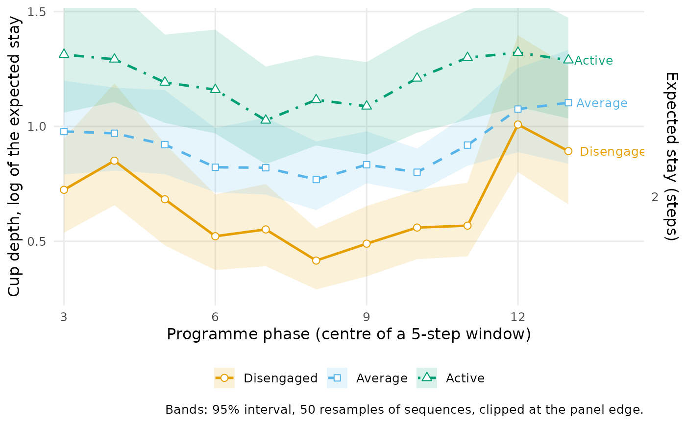
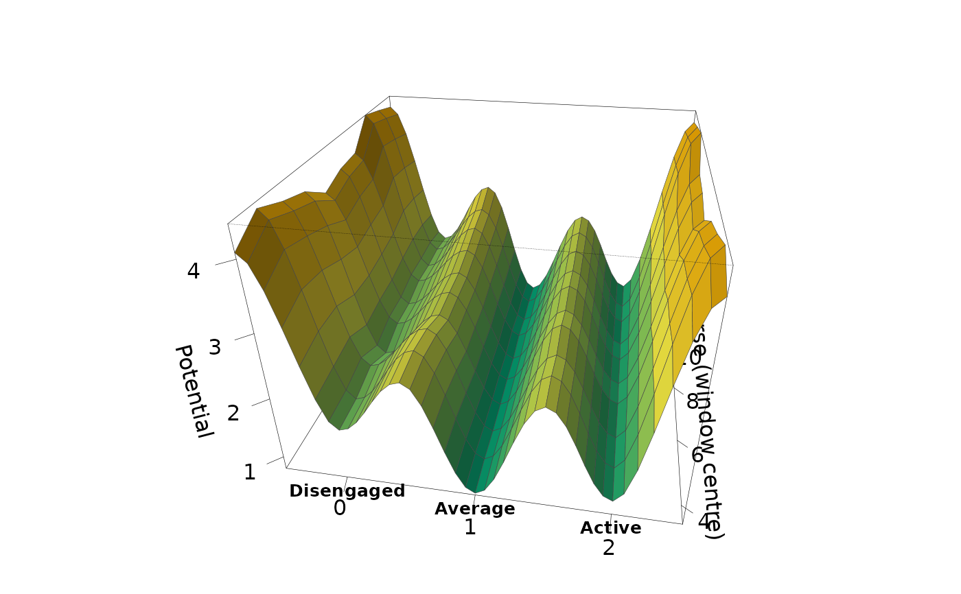
plot()method:"lines"(default) draws one line per state with its interval band, the states told apart by colour, point shape, line type and a label at the end of each line;"surface"draws a 3Dgraphics::persp()landscape with the states across and the second axis in depth, one panel per network on a shared height scale, ridges included withdepth = "occupancy".- theta, phi
For
plot(type = "surface"): the viewing angles. Defaults10and30.
Value
A net_landscape_trend object. print() shows each state's
height at the first and the last window or slice and its range, and
counts the points that could not be estimated; summary() returns the
table below; plot() returns a ggplot with type = "lines", and
with type = "surface" draws the landscape and returns its input
invisibly. print() returns its input invisibly.
summary() returns a data frame with one row per network, position and
feature: group, along, value (window centre or covariate value),
label (window steps or value), feature ("well", or "ridge" with
depth = "occupancy"), state (a state, or two for a ridge), the height
(depth for "stay", potential for "occupancy"), ci_lower,
ci_upper, n_from (transitions out of the state in the window, or
their weighted sum in the slice; wells only) and dwell ("stay"
only).
The object's fields:
- table
The table
summary()returns.- states, groups
The states in drawing order and the network names (
"network"for a single one).- along, depth, window, k, iter, ci_level
The settings used.
Details
Network input replays the network's per-sequence weighting, concatenation
and boundary markers, and the concatenated sequences are the resampling
units. With a covariate, its value must be constant within each
concatenated unit. Scaled, thresholded or otherwise modified networks
whose weights do not match their stored sequences are refused; pass the
original sequences to estimate a new landscape. In a network built with
params = list(weighted = TRUE), the transitions of a phase window keep
the weight of their whole sequence.
With depth = "stay", a window or slice in which a state is never left
gives an infinite depth, and one in which it does not occur gives NA.
With depth = "occupancy", ridges join the states next to each other in
states order and the last state to the first (one ridge with two
states); a window whose chain has no unique stationary distribution is
NA throughout, and a ridge never crossed is NA. Such points are kept
in summary(), left out of the lines and the surface, and counted in the
plot caption. Interval bands are clipped at the panel edge, which is set
by the estimates.
Along a covariate, sequences without its value or with fewer than two
observed positions are left out, and the kernel's half-width is the distance
to the k-th nearest sequence, but at least 1/50 of the covariate's
range.
Errors
nestimate_not_markov for a network that is not a transition network;
nestimate_bad_input for an unknown, non-numeric or constant covariate,
a covariate that varies within a concatenated sequence, bad states, a
window longer than the sequences, input without sequences, or a network
whose weights cannot be rebuilt from its sequences (a scaled or
thresholded one included); nestimate_landscape_unestimable for fewer
than five usable sequences along a covariate.
References
Cleveland, W. S. (1979). Robust locally weighted regression and smoothing scatterplots. Journal of the American Statistical Association, 74, 829–836.
Kramers, H. A. (1940). Brownian motion in a field of force and the diffusion model of chemical reactions. Physica, 7, 284–304.
Wang, J., Xu, L., & Wang, E. (2008). Potential landscape and flux framework of nonequilibrium networks. PNAS, 105, 12271–12276.
Examples
net <- build_network(trajectories, method = "relative")
trend <- landscape_trend(net, along = "phase",
states = c("Disengaged", "Average", "Active"), iter = 50, seed = 1)
trend
#> Stability landscape along programme phase (5-step windows): 3 states, 1 network, 50 resamples
#>
#> Cup depth (log of the expected stay; higher = more stable) at the two ends and its range:
#> state first at_first last at_last min max
#> Disengaged 1-5 0.72 11-15 0.89 0.42 1.01
#> Average 1-5 0.98 11-15 1.10 0.77 1.10
#> Active 1-5 1.31 11-15 1.29 1.03 1.32
# \donttest{
plot(trend)
 occupancy <- landscape_trend(net, depth = "occupancy", window = 6,
states = c("Disengaged", "Average", "Active"), iter = 50, seed = 1)
plot(occupancy, type = "surface")
 # }