Higher-Order Network Analysis with Simplicial Complexes • Nestimate

Introduction

When we analyze sequential data as a network — who follows whom, which state leads to which — we typically build a first-order Markov model: the probability of the next state depends only on the current state. This is the foundation of Transition Network Analysis (TNA).

But human behavior is not always memoryless. Consider two programmers working with an AI coding assistant:

Programmer A: Specify → Request → Specify → Request (a steady back-and-forth)
Programmer B: Frustrate → Specify → Request → Command (escalating from frustration to direct commands)

In a first-order model, both sequences contribute equally to the Specify → Request transition. But the context — what came before — matters. The sequence Frustrate → Specify may lead to very different next actions than Request → Specify. These are higher-order dependencies: cases where the past two (or more) states jointly predict the future better than the current state alone.

This tutorial introduces a complete pipeline for detecting, quantifying, and visualizing higher-order structure in sequential data. We progress from standard transition networks through statistical order detection, pathway analysis, and into the topology of higher-order interactions using simplicial complexes.

What you will learn

Test whether your data has higher-order dependencies (and at what order)
Identify which specific pathways deviate from first-order expectations
Detect anomalously frequent or rare behavioral sequences
Compute topological invariants (Betti numbers, Euler characteristic)
Track how network topology changes across thresholds (persistent homology)
Visualize higher-order pathways as simplicial blob diagrams
Compare higher-order structure across groups

Packages

library(Nestimate)
library(cograph)

# Guard cograph::plot_simplicial() against grDevices::chull() failing on
# degenerate pathway clouds (collinear / single-point), which the CRAN
# cograph (2.1.1) hits but the dev build (>= 2.3.5) fixes in .smooth_blob().
# Shadow the function in the knit env so all call sites fall back to
# splot() with a warning rather than aborting the render. Package code is
# unaffected (scope is this vignette's knit environment only).
plot_simplicial <- function(...) {
  args <- list(...)
  tryCatch(do.call(cograph::plot_simplicial, args),
           error = function(e) {
             warning("plot_simplicial fell back to splot(): ",
                     conditionMessage(e), call. = FALSE)
             splot(args[[1]])
           })
}

cograph provides the simplicial visualization (plot_simplicial()). Nestimate provides the higher-order network construction (build_hon, build_hypa, build_mogen) and simplicial complex analysis (build_simplicial, betti_numbers, persistent_homology, q_analysis).

Building the Network

We use a dataset of human–AI pair programming sessions where a researcher coded each human action into 9 behavioral categories: Request, Specify, Command, Correct, Refine, Verify, Inquire, Interrupt, and Frustrate.

data("human_long", package = "Nestimate")

net <- build_network(human_long, method = "relative",
                     action = "code", actor = "session_id",
                     time = "timestamp")
net

Transition Network (relative probabilities) [directed]
  Weights: [0.018, 0.620]  |  mean: 0.111

  Weight matrix:
            Command Correct Frustrate Inquire Interrupt Refine Request Specify
  Command     0.235   0.088     0.055   0.066     0.035  0.038   0.155   0.280
  Correct     0.093   0.091     0.138   0.057     0.054  0.112   0.120   0.278
  Frustrate   0.103   0.115     0.176   0.075     0.047  0.171   0.111   0.125
  Inquire     0.196   0.126     0.098   0.188     0.094  0.062   0.084   0.106
  Interrupt   0.259   0.081     0.094   0.123     0.102  0.080   0.069   0.122
  Refine      0.058   0.075     0.072   0.047     0.042  0.086   0.146   0.457
  Request     0.096   0.019     0.044   0.067     0.051  0.033   0.039   0.620
  Specify     0.263   0.058     0.081   0.072     0.167  0.074   0.070   0.172
  Verify      0.224   0.079     0.164   0.118     0.043  0.097   0.116   0.083
            Verify
  Command    0.048
  Correct    0.056
  Frustrate  0.077
  Inquire    0.044
  Interrupt  0.069
  Refine     0.018
  Request    0.032
  Specify    0.043
  Verify     0.077

  Initial probabilities:
  Specify       0.679  ████████████████████████████████████████
  Command       0.175  ██████████
  Request       0.055  ███
  Interrupt     0.030  ██
  Correct       0.019  █
  Refine        0.019  █
  Frustrate     0.013  █
  Inquire       0.008
  Verify        0.002

splot(net, minimum = 0.05, title = "Human Actions in AI-Assisted Coding")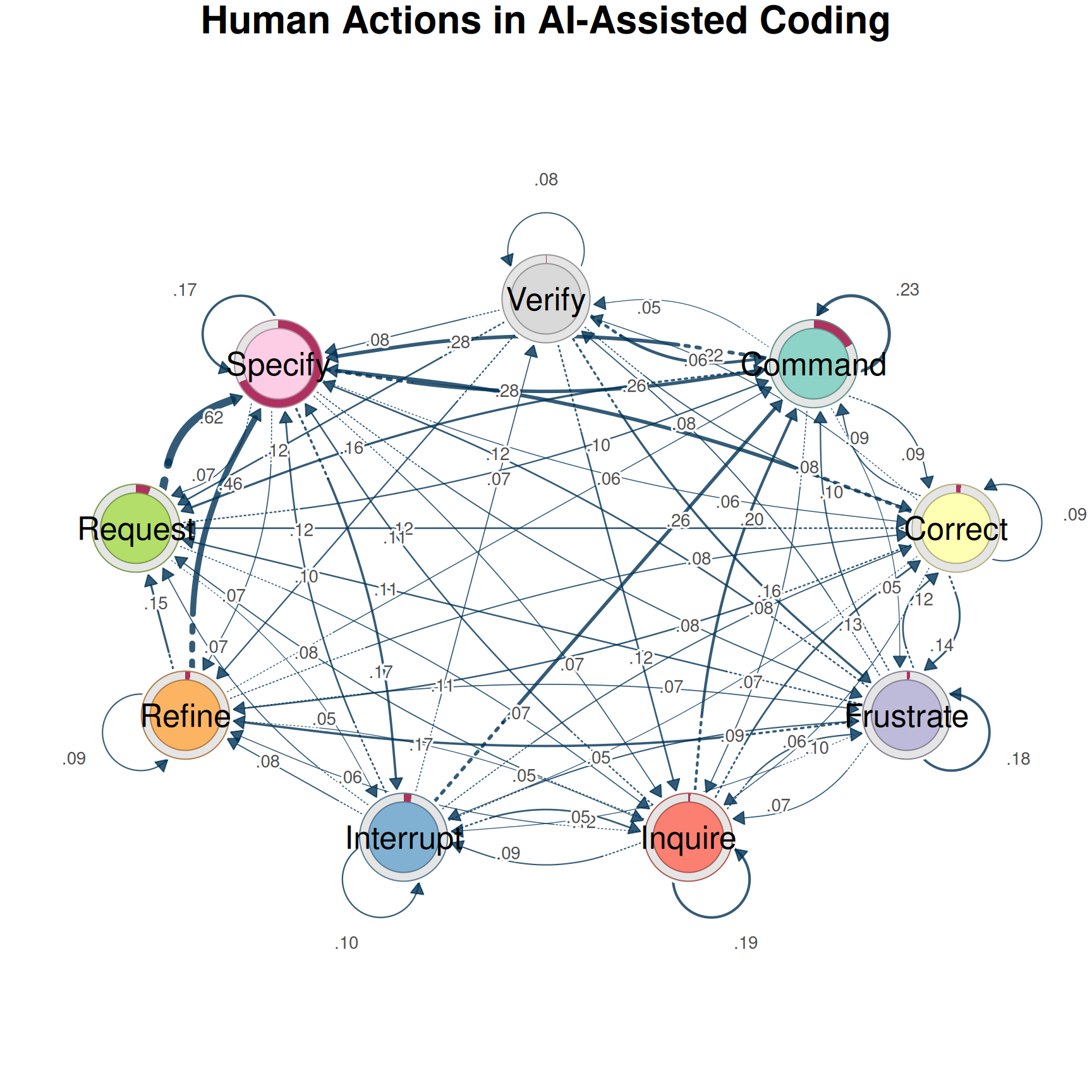

Several patterns stand out: Specify is the hub — most actions lead to and from it. Self-loops on Specify and Command indicate persistence. The Request → Specify → Command backbone reflects the natural workflow. But this first-order view might be hiding important patterns. Does it matter how someone arrived at Specify?

Is First-Order Enough? Multi-Order Model Selection

Before investing in higher-order analysis, we should answer: does sequential memory actually matter? The Multi-Order Generative Model (MOGen; Scholtes 2017) fits Markov models at increasing orders and compares them using information criteria. Higher-order models fit better but have exponentially more parameters — AIC and BIC find the best tradeoff.

mg <- build_mogen(net, max_order = 4)
summary(mg)

Multi-Order Generative Model (MOGen) Summary

  States: Command, Correct, Frustrate, Inquire, Interrupt, Refine, Request, Specify, Verify
  Paths: 508 | Observations: 10778
  Best by AIC: order 4  |  Best by BIC: order 1
  Selected:    order 4 (by aic)

        order layer_dof cum_dof    loglik      aic      bic best selected
order_0     0         8       8 -22001.20 44018.40 44076.68
order_1     1        72      80 -20805.61 41771.23 42354.05  BIC
order_2     2       621     701 -19819.55 41041.10 46148.07
order_3     3      2445    3146 -17152.10 40596.20 63515.63
order_4     4      2990    6136 -11469.73 35211.46 79913.83  AIC      <--

plot(mg)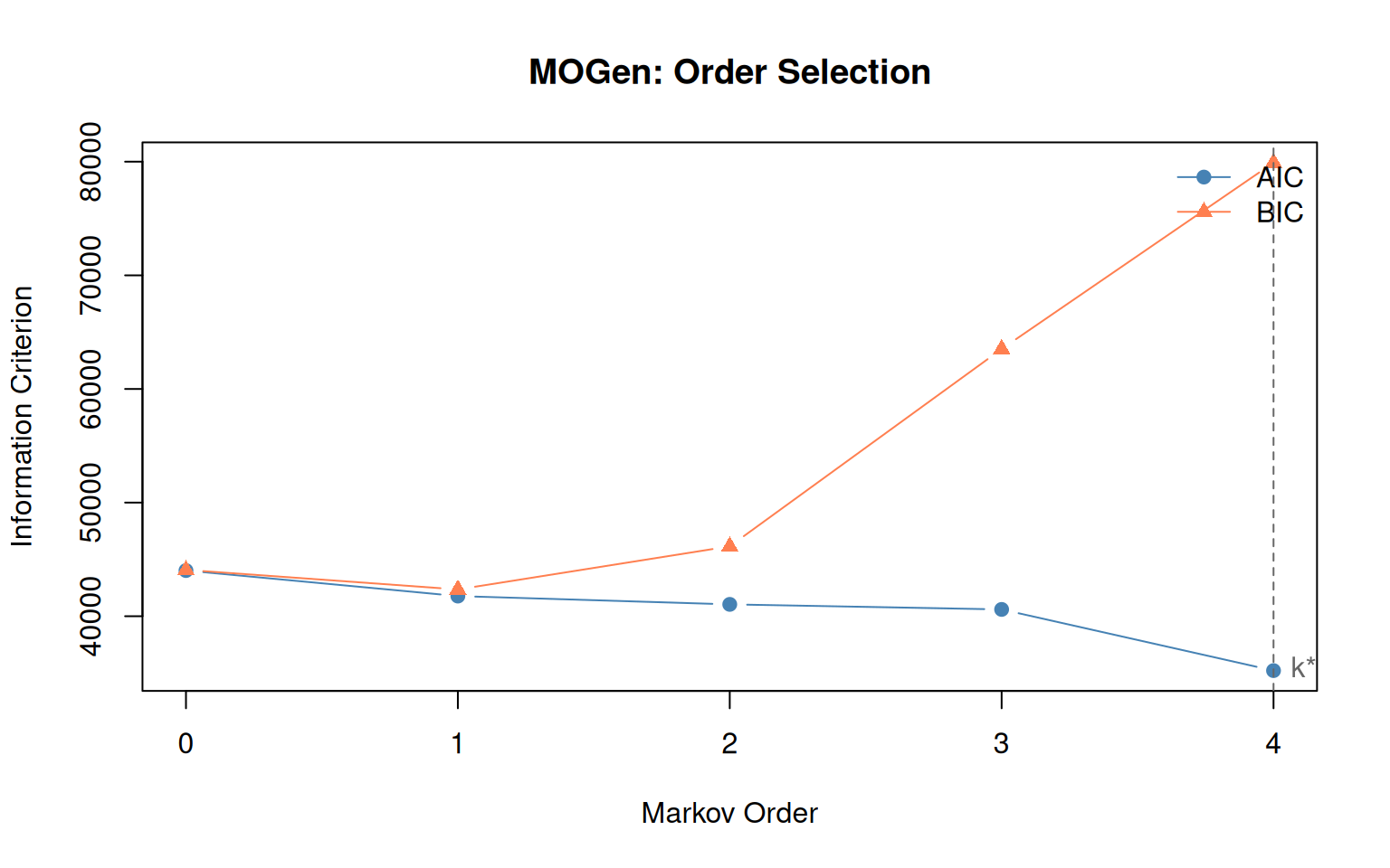

The plot traces AIC and BIC as functions of the Markov order. Because higher-order models always fit better in terms of raw log-likelihood (their parameter space contains the lower-order one), the meaningful comparison is between fit and complexity. AIC penalises each parameter by 2; BIC penalises by log(n), which for this dataset is much larger than 2 — so BIC favors small orders much more aggressively than AIC.

Interpreting the results

Order 0: Actions are independent — no sequential structure.
Order 1: The standard Markov model is sufficient.
Order 2+: Higher-order dependencies exist. A first-order TNA would miss them.

Even when order 1 is globally optimal (by BIC), specific pathways may still exhibit higher-order behavior — the global model averages over all states. The HON analysis below detects these local patterns. The next section adds a complementary, principled hypothesis test that often reveals signal BIC is too parsimonious to flag.

Second-order transition matrix

mogen_transitions() extracts the transitions at a given order, showing which two-step contexts lead to different outcomes:

mt <- mogen_transitions(mg, order = 2)
mt[1:8, ]

                             path count probability               from
1   Specify -> Command -> Specify   281      0.3914 Specify -> Command
2   Command -> Request -> Specify   228      0.7782 Command -> Request
3   Specify -> Command -> Request   198      0.2758 Specify -> Command
4 Request -> Specify -> Interrupt   187      0.3264 Request -> Specify
5   Command -> Command -> Command   163      0.3800 Command -> Command
6 Command -> Specify -> Interrupt   148      0.2792 Command -> Specify
7   Specify -> Request -> Specify   124      0.6526 Specify -> Request
8    Specify -> Refine -> Specify   122      0.6010  Specify -> Refine
         to
1   Specify
2   Specify
3   Request
4 Interrupt
5   Command
6 Interrupt
7   Specify
8   Specify

Each row is a second-order pathway. The from column is the two-state context, to is the predicted next state, count is the empirical frequency, and probability is the conditional P(to | from). A high count combined with a high probability is a predictive context: knowing the previous two states pins down the next one. A high count with low probability is a common but ambiguous context — frequent in the data, but its successor distribution is spread out.

plot_simplicial() accepts the mogen_transitions() data.frame directly. It takes the top pathways by count and renders each as a smooth blob over a shared circular layout, with the path’s intermediate states in blue and the target state in red. Repeated states (like Specify -> Command -> Specify) get distinct positions so the blob covers three visually distinct nodes rather than collapsing to a line.

plot_simplicial(net, pathways = mt, max_pathways = 6,
                title = "Top 6 second-order pathways")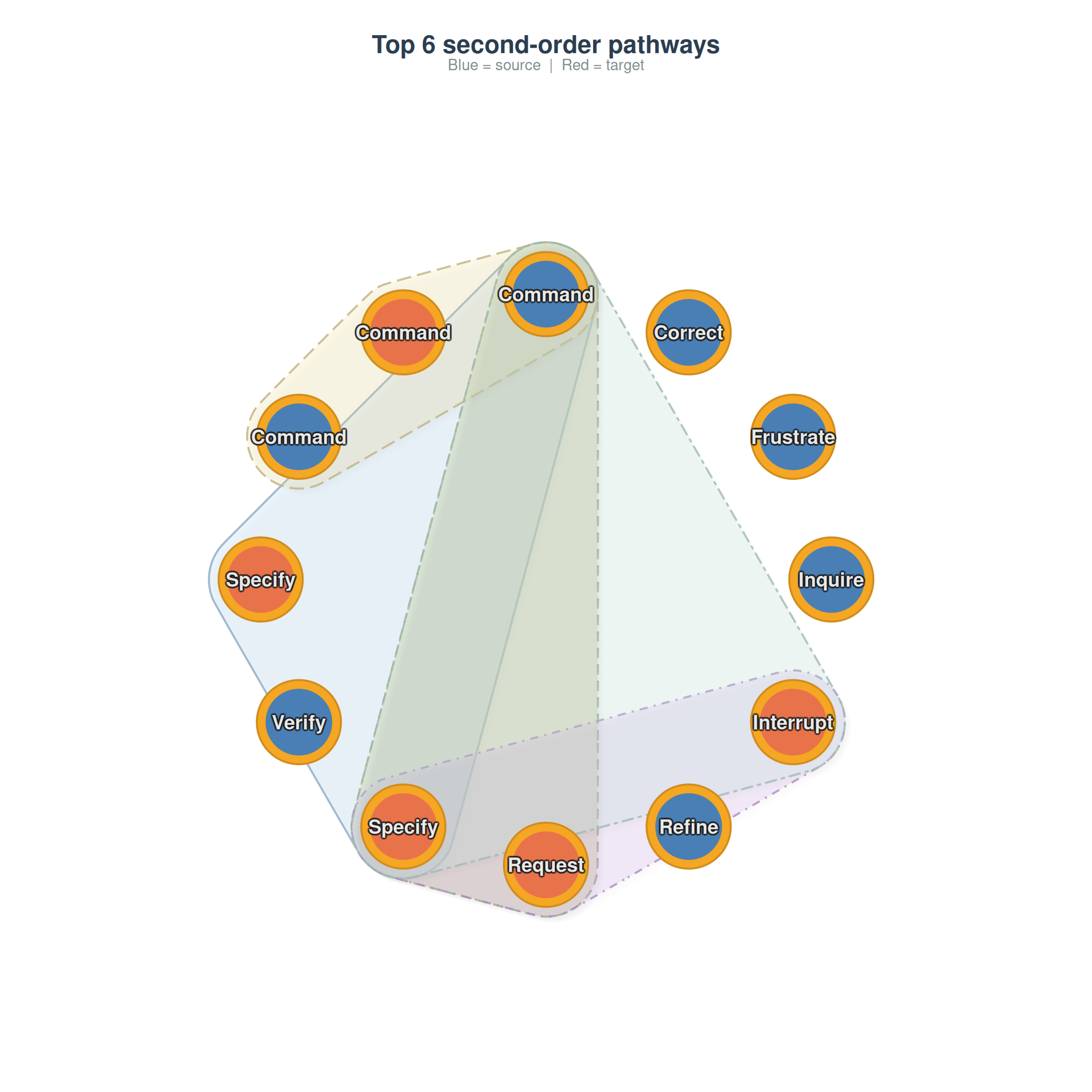

To zoom in on the single most frequent pathway, set max_pathways = 1 and let the data.frame drive the selection. Because mogen_transitions() returns rows already sorted by count, max_pathways = N always picks the top N:

plot_simplicial(net, pathways = mt, max_pathways = 1)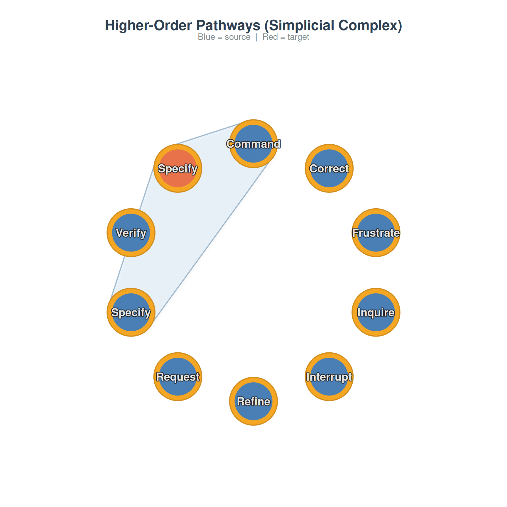

Permutation-exact Markov order test

MOGen uses information criteria. A complementary, principled approach is the permutation-exact LRT in markov_order_test(): at each order $k$ , it tests $H_0$ : “process is order $(k-1)$ ” against $H_1$ : “process is order $k$ ” by reframing as a conditional-independence test on $(k+1)$ -grams. The null distribution is built by shuffling successor labels within each context — so the test is exact under $H_0$ , with no plug-in MLE bias from sparse $(k+1)$ -gram tables.

mot <- markov_order_test(net, max_order = 3, n_perm = 200, seed = 1)
mot

Markov Order Test  [within-w permutation, n_perm = 200, alpha = 0.050]
  508 sequences / 10778 observations / 9 states

  Selected order  BIC: 1   AIC: 3   permutation-LRT: 3

 order    loglik      AIC      BIC   df      g2 p_permutation  p_asymptotic
     0 -22001.20 44018.40 44076.68   NA      NA            NA            NA
     1 -20805.61 41771.23 42354.05   64 2365.38   0.004975124  0.000000e+00
     2 -19819.55 41041.10 46148.07  576 1817.12   0.004975124 1.702866e-128
     3 -17152.10 40596.20 63515.63 4706 5163.79   0.004975124  2.317583e-06
 significant
          NA
        TRUE
        TRUE
        TRUE

plot(mot)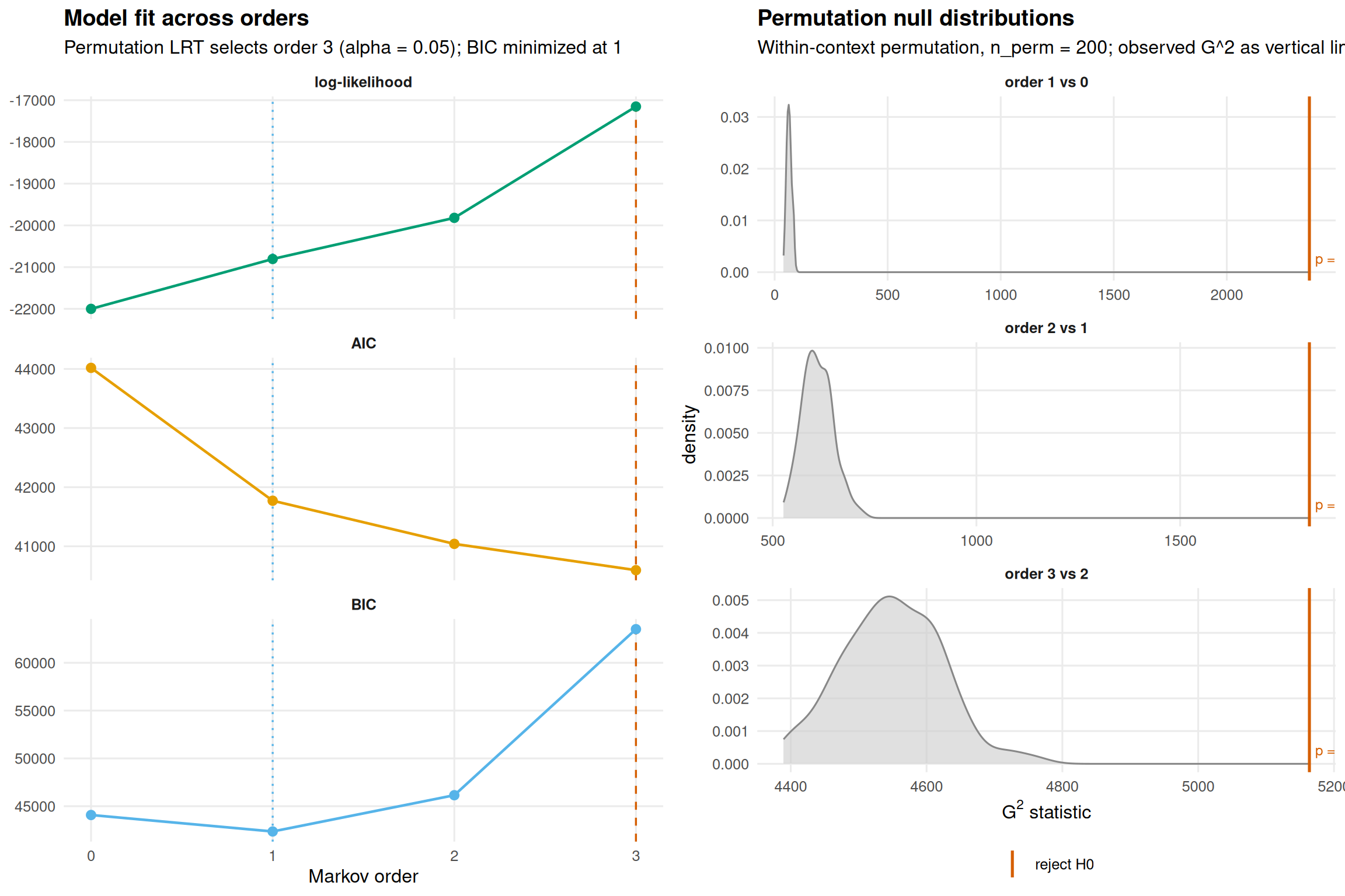

The output reveals a tension that is hidden by any single criterion. BIC selects the smallest order (heavy parsimony penalty). AIC and the permutation LRT both flag higher orders as significantly better — every increase in order yields a $G^2$ statistic far in the tail of the within-context permutation null. The right panel makes this concrete: the grey density is the null $G^2$ distribution per order, and the colored vertical line is the observed value. When the line sits in the right tail, $H_0$ is rejected and the higher order carries genuine information beyond the previous one.

The takeaway: sequential memory exists in this dataset. BIC penalises it because the parameter space at order 3 is enormous (4,706 degrees of freedom for the order-3 test alone), but the data does pay the cost.

Per-state predictability: transition entropy

Order-selection answers a global question. Transition entropy answers a per-state question: how predictable is each state’s next move? transition_entropy() computes the Shannon row-entropy H(P[i, ]) = -sum_j P[i,j] log P[i,j] for every state, the chain-level entropy rate h(P) = sum_i pi_i H(P[i, ]) (the Shannon-McMillan-Breiman per-step uncertainty under the stationary distribution pi), and the redundancy H(pi) - h(P) (how much the previous state reduces uncertainty about the next).

te <- transition_entropy(net)
te

Transition Entropy (9 states, bits; ceiling = 3.170)

                          raw            normalised
  Entropy rate    h(P)  = 2.815 bits    0.888
  Stationary    H(pi)  = 2.983 bits    0.941
  Redundancy   H(pi)-h = 0.167 bits    0.056

Normalised: h(P) and H(pi) are raw / log_2(n_states) (0 = deterministic, 1 = uniform);
  redundancy is the relative redundancy (H(pi) - h(P)) / H(pi), not raw / log_2(n_states).

plot(te)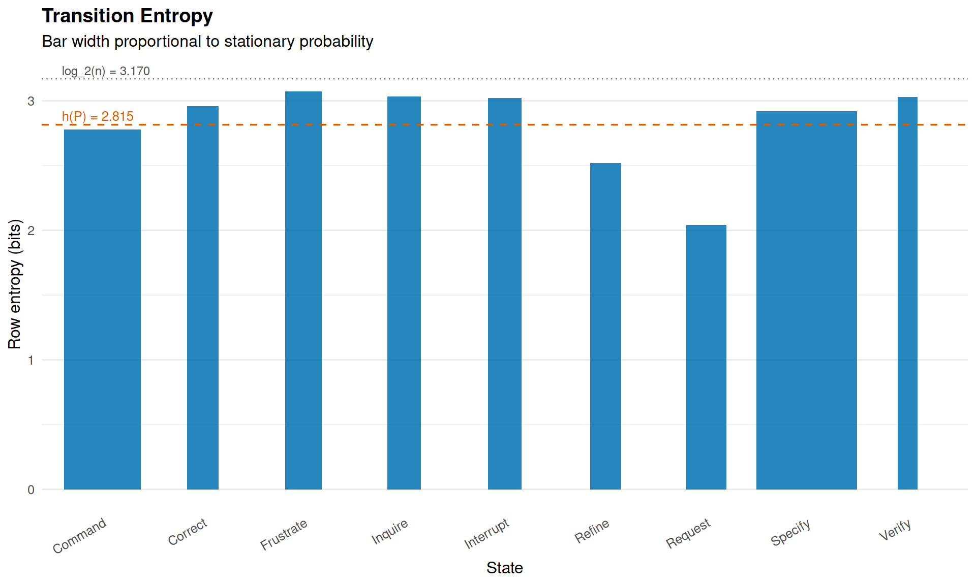

Each bar is a state’s outgoing-distribution entropy in bits; the bar’s width is proportional to the stationary probability, so the visual area sums to the entropy rate h(P). The dashed red line marks h(P); the dotted line marks the ceiling log_2(n) where every state has a uniform outgoing distribution. States whose bar pokes near the ceiling are unpredictable hubs (their next state is essentially random); short bars are deterministic — once you arrive there, the next step is largely fixed.

Higher-Order Networks (HON)

While MOGen tells us whether higher-order dependencies exist on average, the Higher-Order Network (HON; Xu et al. 2016) tells us where. HON tests, for each state, whether adding context significantly changes the outgoing transition distribution using KL-divergence. If the distribution after Request → Specify differs from Frustrate → Specify, HON creates separate nodes for these contexts.

hon <- build_hon(net)
hon

Higher-Order Network (HON)
  Nodes:        977 (9 first-order states)
  Edges:        3733
  Max order:    5 (requested 5)
  Min freq:     1
  Trajectories: 508

pathways(hon, top = 10)

 [1] "Specify Command -> Specify"
 [2] "Command Request -> Specify"
 [3] "Specify Command -> Request"
 [4] "Request Specify -> Interrupt"
 [5] "Specify Command Request -> Specify"
 [6] "Command Command -> Command"
 [7] "Command Specify -> Interrupt"
 [8] "Command Request Specify -> Interrupt"
 [9] "Specify Command Specify -> Interrupt"
[10] "Specify Request -> Specify"

Out of 3733 total edges, 3652 (98%) are higher-order — transitions where the preceding context changes the outcome. Look for pathways where the higher-order probability differs substantially from the first-order probability — these represent genuine contextual effects.

Raw path frequencies

The most common 3-step sequences regardless of statistical significance:

path_counts(net, k = 3, top = 15)

                              path count proportion
1    Specify -> Command -> Specify   281     0.0288
2    Command -> Request -> Specify   228     0.0234
3    Specify -> Command -> Request   198     0.0203
4  Request -> Specify -> Interrupt   187     0.0192
5    Command -> Command -> Command   163     0.0167
6  Command -> Specify -> Interrupt   148     0.0152
7    Specify -> Request -> Specify   124     0.0127
8     Specify -> Refine -> Specify   122     0.0125
9    Specify -> Specify -> Specify   121     0.0124
10 Specify -> Interrupt -> Command   109     0.0112
11   Command -> Specify -> Command   106     0.0109
12   Request -> Specify -> Specify    94     0.0096
13   Specify -> Command -> Command    93     0.0095
14   Command -> Specify -> Specify    76     0.0078
15   Specify -> Specify -> Command    76     0.0078

Path Anomaly Detection (HYPA)

HON detects where higher-order structure exists. HYPA (LaRock et al. 2020) takes a complementary approach: it detects which specific paths occur significantly more or less often than expected under a null model.

HYPA constructs a De Bruijn graph and computes expected path frequencies using a multi-hypergeometric null model: given the in- and out-degrees of every node in the De Bruijn graph, what is the chance distribution over path frequencies if the edges were assigned uniformly at random subject to those degree constraints? Paths whose observed frequency falls in the upper or lower tail of this null are flagged:

Over-represented paths occur far more often than the degree-preserving null predicts. They represent learned behavioural routines — sequences the actors return to more reliably than their constituent transitions alone would suggest.
Under-represented paths are systematically avoided — observed far less than chance. They reveal sequences that are pragmatically discouraged: cognitively redundant, socially inappropriate, or practically ineffective for the task at hand.

hypa <- build_hypa(net)
hypa

HYPA: Path Anomaly Detection
  Order(s):     2
  Edges:        702
  Anomalous:    177 (alpha=0.05, p_adjust=BH)
    Over-repr:  133
    Under-repr: 44

plot_simplicial(hypa, dismantled = TRUE)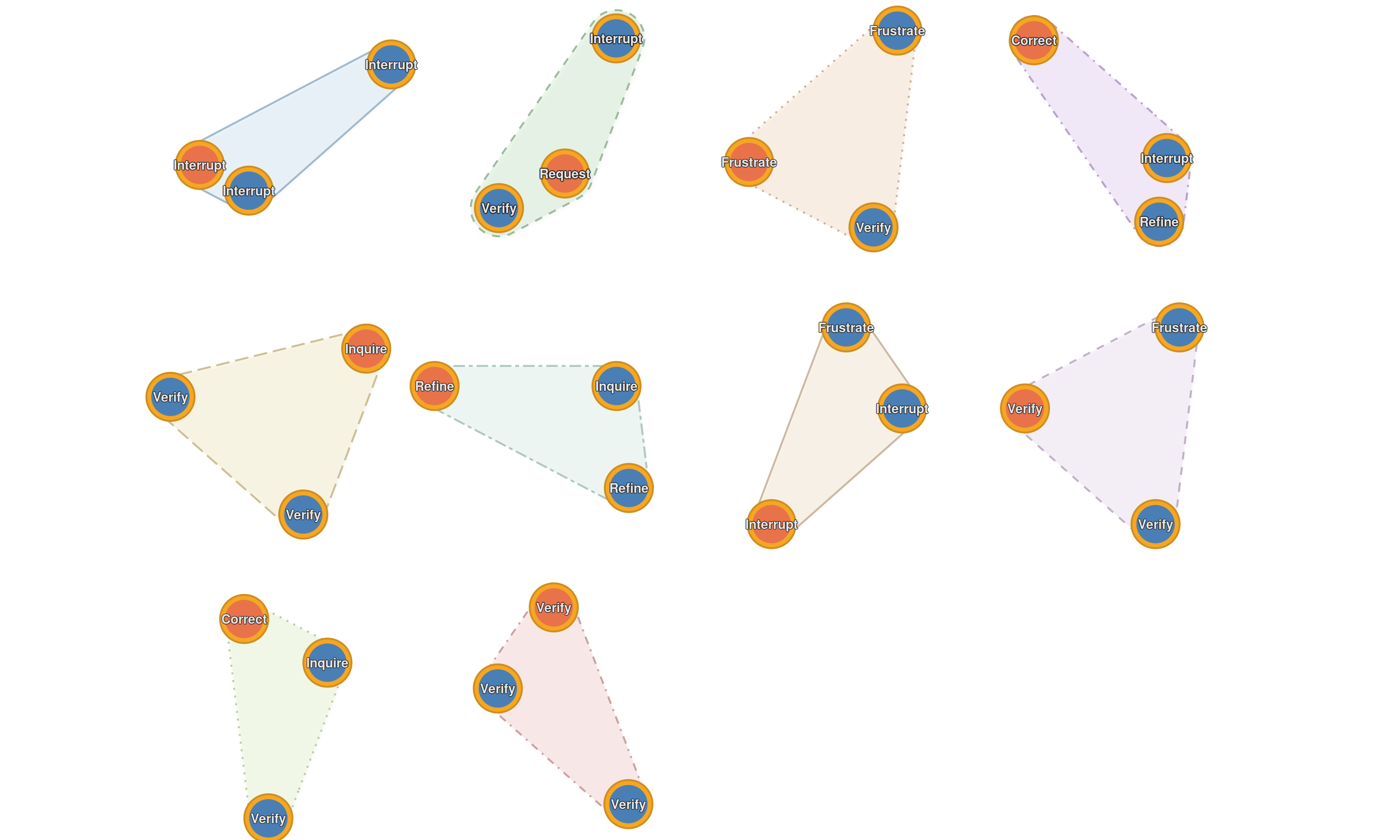

Over-represented pathways

Top over-represented paths sorted by ratio (observed / expected):

summary(hypa, type = "over", order_by = "ratio", n = 8)

HYPA Summary

  Order(s): 2 | Edges: 702
  Alpha: 0.05 | p_adjust: BH
  Anomalous: 177 (over: 133, under: 44) | order_by: ratio

  Over-represented (top 8 ):
                                path observed  expected     ratio       p_tail
 Interrupt -> Interrupt -> Interrupt       29 2.7844871 10.414844 5.398941e-20
      Verify -> Interrupt -> Request        5 0.6879572  7.267894 7.213367e-04
    Frustrate -> Verify -> Frustrate       27 3.8139380  7.079297 1.082539e-14
      Refine -> Interrupt -> Correct        6 0.8519593  7.042590 2.547426e-04
         Verify -> Verify -> Inquire       10 1.4568505  6.864122 3.120114e-06
         Refine -> Inquire -> Refine        8 1.2069424  6.628320 3.795876e-05
 Interrupt -> Frustrate -> Interrupt       12 2.0454124  5.866788 1.679456e-06
       Verify -> Frustrate -> Verify       22 3.9821999  5.524584 3.057447e-10

  order                                path observed  expected     ratio
1     2 Interrupt -> Interrupt -> Interrupt       29 2.7844871 10.414844
2     2      Verify -> Interrupt -> Request        5 0.6879572  7.267894
3     2    Frustrate -> Verify -> Frustrate       27 3.8139380  7.079297
4     2      Refine -> Interrupt -> Correct        6 0.8519593  7.042590
5     2         Verify -> Verify -> Inquire       10 1.4568505  6.864122
6     2         Refine -> Inquire -> Refine        8 1.2069424  6.628320
7     2 Interrupt -> Frustrate -> Interrupt       12 2.0454124  5.866788
8     2       Verify -> Frustrate -> Verify       22 3.9821999  5.524584
        p_tail direction
1 5.398941e-20      over
2 7.213367e-04      over
3 1.082539e-14      over
4 2.547426e-04      over
5 3.120114e-06      over
6 3.795876e-05      over
7 1.679456e-06      over
8 3.057447e-10      over

In this dataset the top-ratio over-represented paths are typically frustration cascades and inquiry-correction loops — composite routines built from transitions that are individually unremarkable but, when chained, occur many times more often than their degrees alone would suggest.

plot_simplicial(hypa, anomaly = "over", dismantled = TRUE) renders one panel per anomalous path so each routine is visible without overlap. Pathways are ranked by ratio, so the most extreme over-representations appear first:

plot_simplicial(hypa, anomaly = "over", max_pathways = 9,
                dismantled = TRUE, ncol = 3)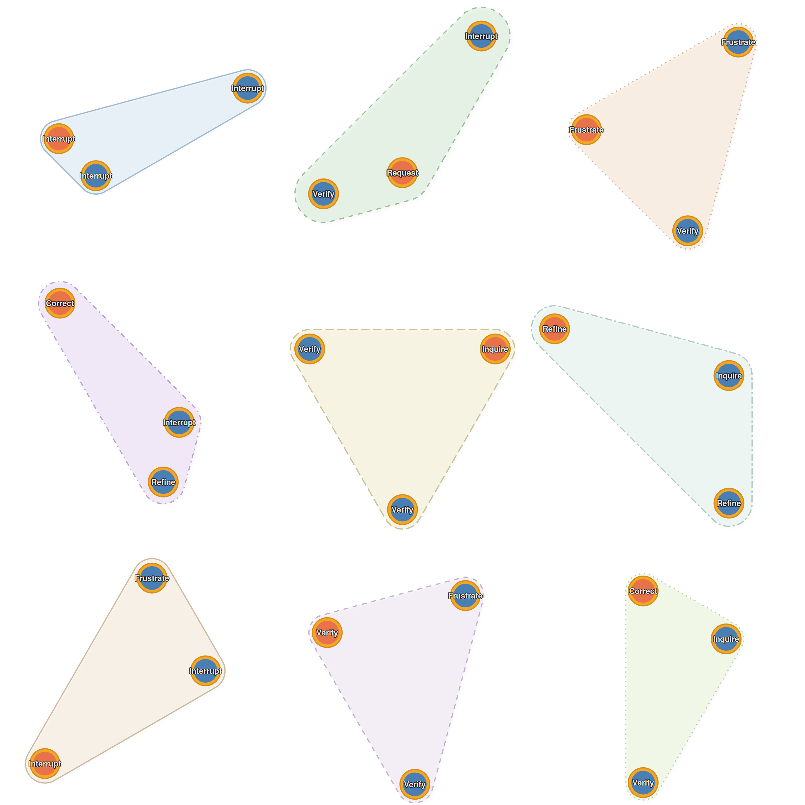

Under-represented pathways

Paths the data actively avoids. The ratios here are typically far from 1.0 in the other direction: observed counts are a fraction of expected, often with very small p-values:

summary(hypa, type = "under", order_by = "ratio", n = 8)

HYPA Summary

  Order(s): 2 | Edges: 702
  Alpha: 0.05 | p_adjust: BH
  Anomalous: 177 (over: 133, under: 44) | order_by: ratio

  Under-represented (top 8 ):
                              path observed  expected     ratio       p_tail
   Inquire -> Specify -> Interrupt        5  27.55236 0.1814726 1.677120e-07
   Frustrate -> Specify -> Command        6  30.26160 0.1982711 9.146340e-08
   Specify -> Specify -> Interrupt       34 148.58597 0.2288238 4.453897e-30
 Frustrate -> Specify -> Interrupt        9  36.40848 0.2471951 5.990496e-08
   Specify -> Command -> Interrupt        8  31.60485 0.2531257 5.922403e-07
   Frustrate -> Command -> Request        5  19.18825 0.2605761 1.313412e-04
    Refine -> Specify -> Interrupt       31 112.17749 0.2763478 7.847657e-20
       Refine -> Specify -> Verify        8  28.65139 0.2792185 5.388930e-06

  order                              path observed  expected     ratio
1     2   Inquire -> Specify -> Interrupt        5  27.55236 0.1814726
2     2   Frustrate -> Specify -> Command        6  30.26160 0.1982711
3     2   Specify -> Specify -> Interrupt       34 148.58597 0.2288238
4     2 Frustrate -> Specify -> Interrupt        9  36.40848 0.2471951
5     2   Specify -> Command -> Interrupt        8  31.60485 0.2531257
6     2   Frustrate -> Command -> Request        5  19.18825 0.2605761
7     2    Refine -> Specify -> Interrupt       31 112.17749 0.2763478
8     2       Refine -> Specify -> Verify        8  28.65139 0.2792185
        p_tail direction
1 1.677120e-07     under
2 9.146340e-08     under
3 4.453897e-30     under
4 5.990496e-08     under
5 5.922403e-07     under
6 1.313412e-04     under
7 7.847657e-20     under
8 5.388930e-06     under

Notice paths like Specify -> Specify -> Specify -> Specify — a four-step run of pure specification — appear at a small fraction of expected frequency. The transition Specify -> Specify exists in the data, but stacking it four deep is something programmers actively don’t do. The under-represented set captures these negative sequential constraints.

plot_simplicial(hypa, anomaly = "under", max_pathways = 6,
                dismantled = TRUE, ncol = 3)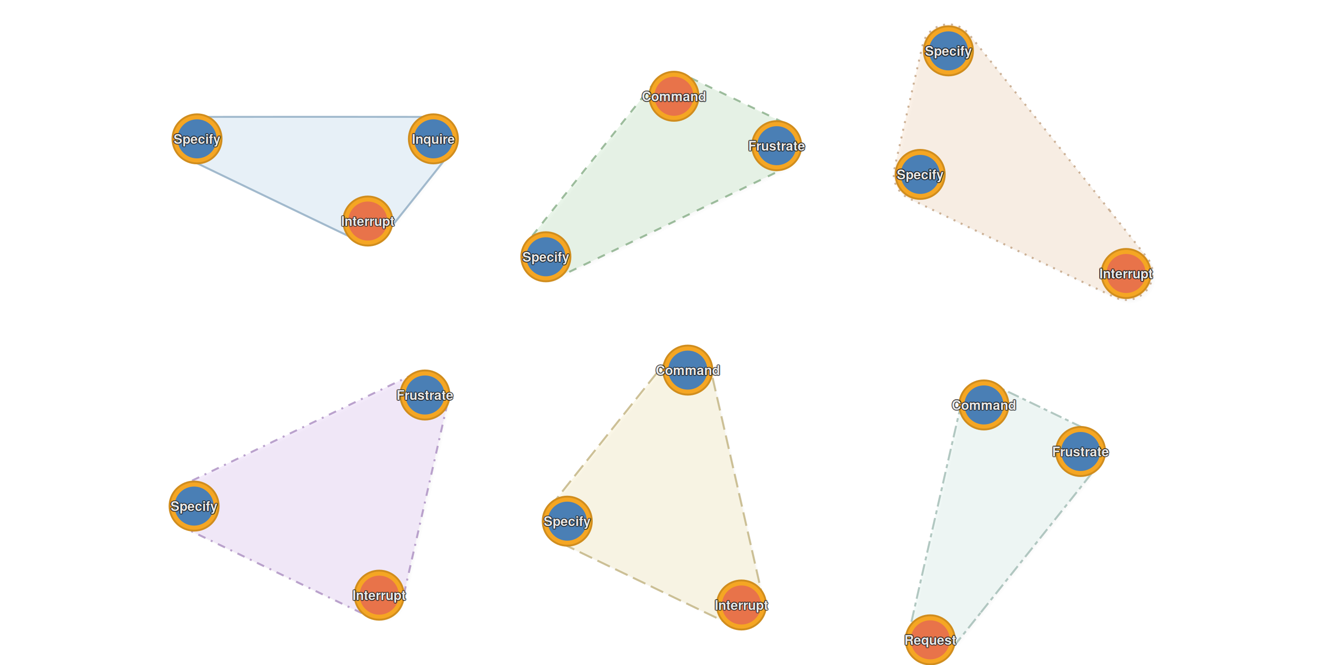

Combined overlay

Multiple pathways on a single plot — overlapping regions indicate states that participate in many higher-order patterns:

plot_simplicial(net, max_pathways = 6,
                title = "Top 6 Higher-Order Pathways")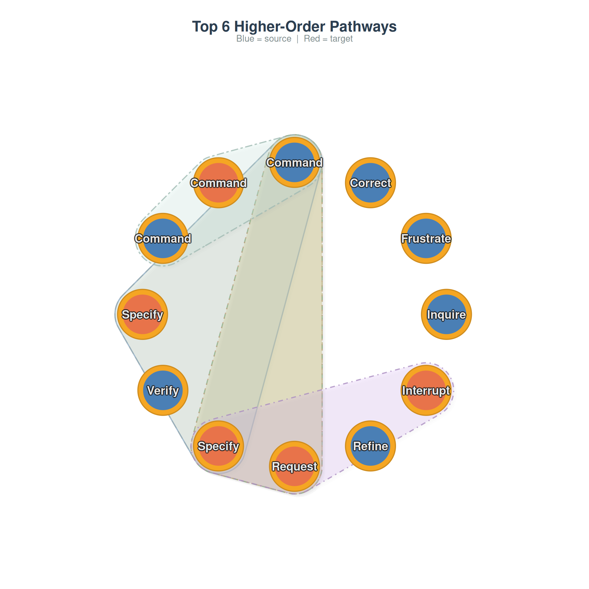

Higher-Order Analysis Across Groups

A powerful application is comparing higher-order structure across conditions. We build grouped networks by cluster (Directive, Evaluative, Metacognitive) and run HYPA on each:

grp_net <- build_network(human_long, method = "relative",
                         action = "code", actor = "session_id",
                         time = "timestamp", group = "cluster")

hypa_results <- lapply(names(grp_net), function(nm) {
  h <- build_hypa(grp_net[[nm]])
  data.frame(
    group = nm,
    total_edges = h$n_edges,
    anomalous = h$n_anomalous,
    over = h$n_over,
    under = h$n_under,
    pct_anomalous = round(100 * h$n_anomalous / h$n_edges, 1)
  )
})
do.call(rbind, hypa_results)

          group total_edges anomalous over under pct_anomalous
1     Directive          27        22   11    11          81.5
2 Metacognitive           8         7    4     3          87.5
3    Evaluative          64        13    9     4          20.3

Groups with a higher percentage of anomalous pathways have more higher-order structure — their sequential dynamics are less predictable from first-order transitions alone.

par(mfrow = c(1, 2))
plot_simplicial(grp_net$Directive, max_pathways = 4,
                title = "Directive: Higher-Order Pathways")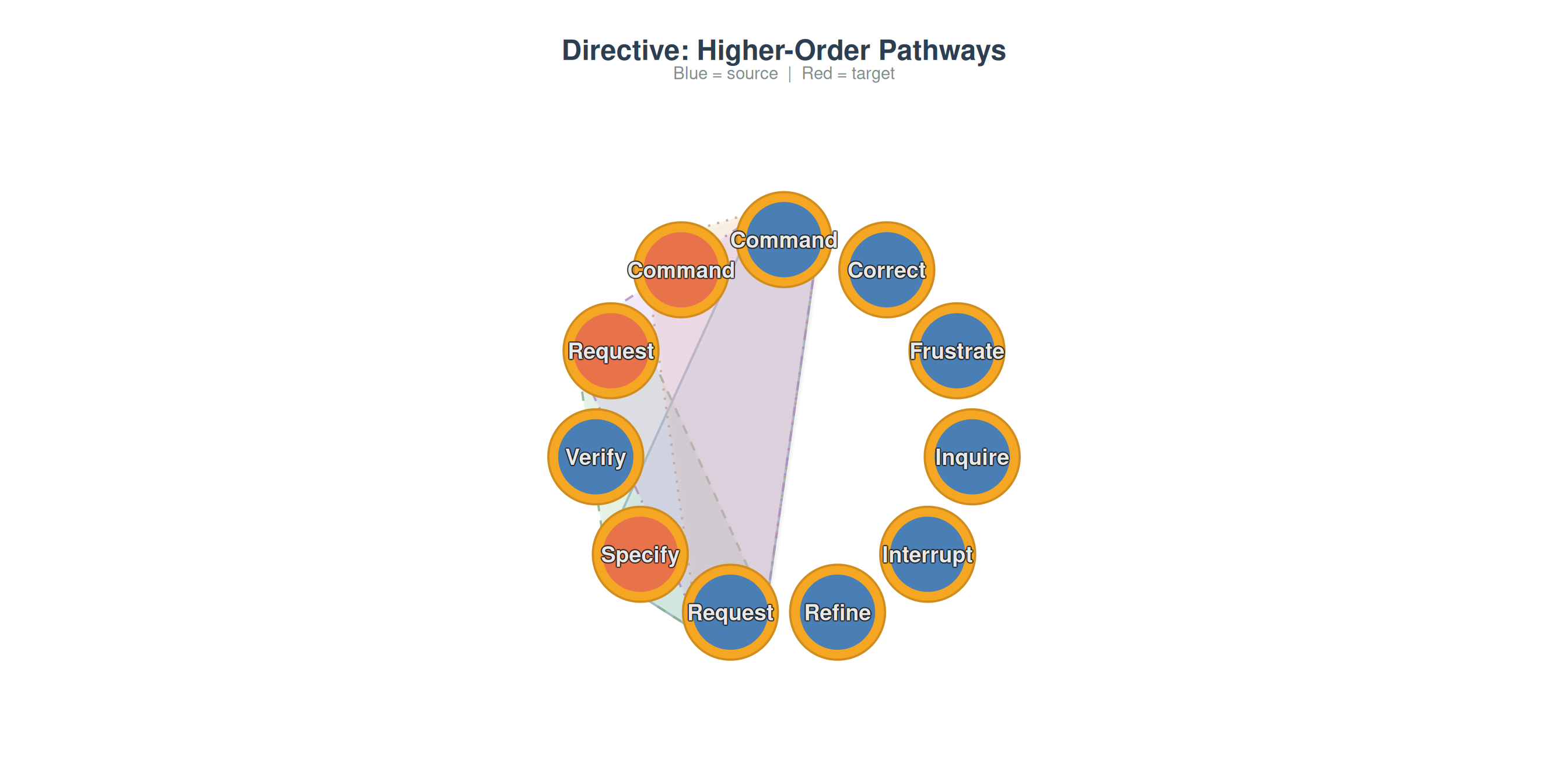

plot_simplicial(grp_net$Evaluative, max_pathways = 4,
                title = "Evaluative: Higher-Order Pathways")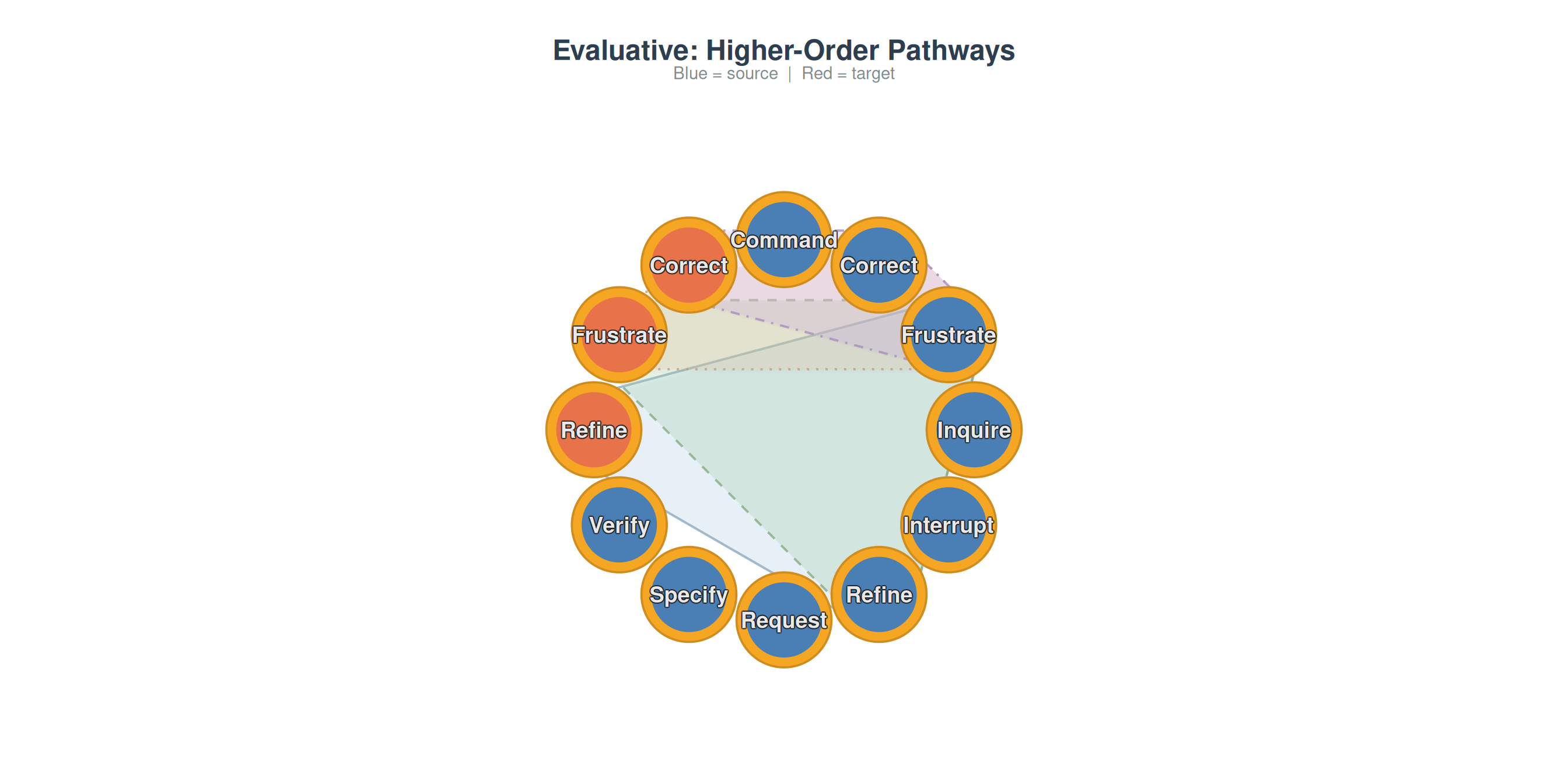

Comparing Datasets

Higher-order analysis is particularly informative when applied to different datasets. Here we compare the human-AI coding data with a collaborative regulation dataset:

data("group_regulation_long", package = "Nestimate")
net_reg <- build_network(group_regulation_long, method = "relative",
                         action = "Action", actor = "Actor")

hypa_coding <- build_hypa(net)
hypa_reg <- build_hypa(net_reg)

comparison <- data.frame(
  dataset = c("Human-AI Coding", "Collaborative Regulation"),
  nodes = c(net$n_nodes, net_reg$n_nodes),
  total_paths = c(hypa_coding$n_edges, hypa_reg$n_edges),
  anomalous = c(hypa_coding$n_anomalous, hypa_reg$n_anomalous),
  over = c(hypa_coding$n_over, hypa_reg$n_over),
  under = c(hypa_coding$n_under, hypa_reg$n_under)
)
comparison

                   dataset nodes total_paths anomalous over under
1          Human-AI Coding     9         702       177  133    44
2 Collaborative Regulation     9         574       229  174    55

par(mfrow = c(1, 2))
plot_simplicial(net, max_pathways = 4,
                title = "Human-AI Coding")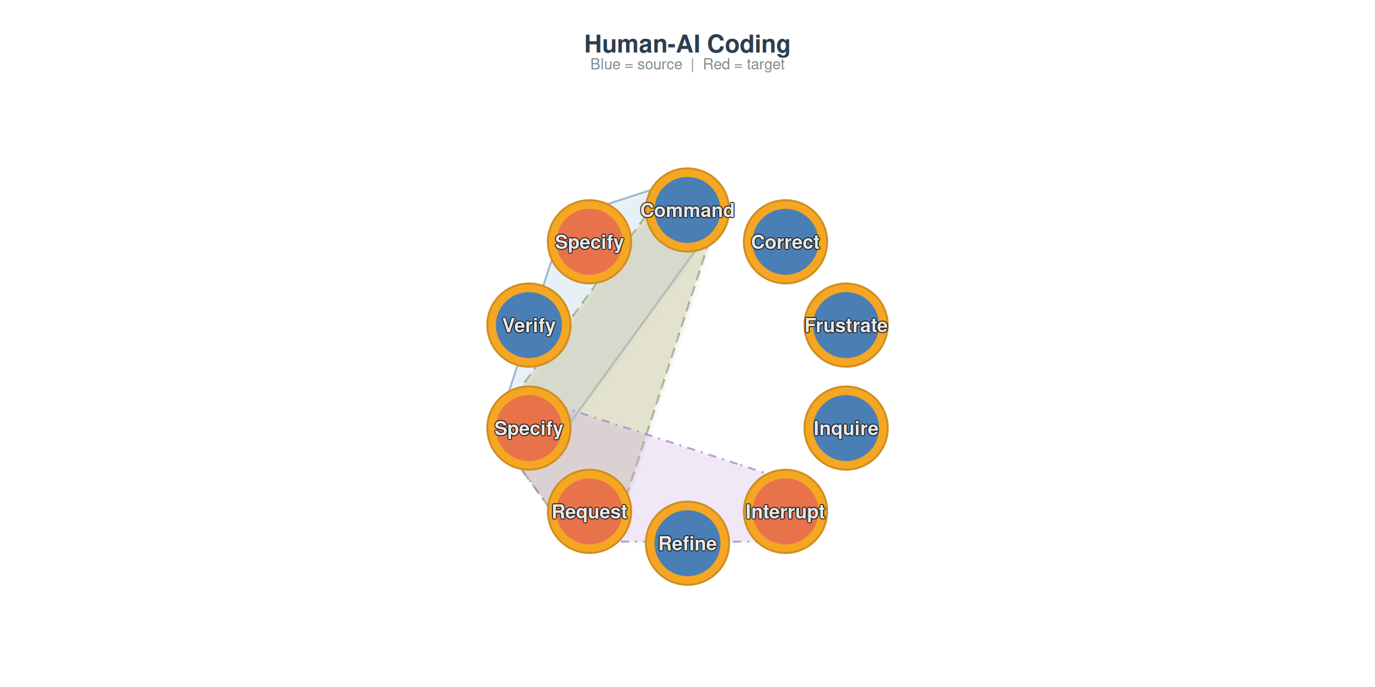

plot_simplicial(net_reg, max_pathways = 4,
                title = "Collaborative Regulation")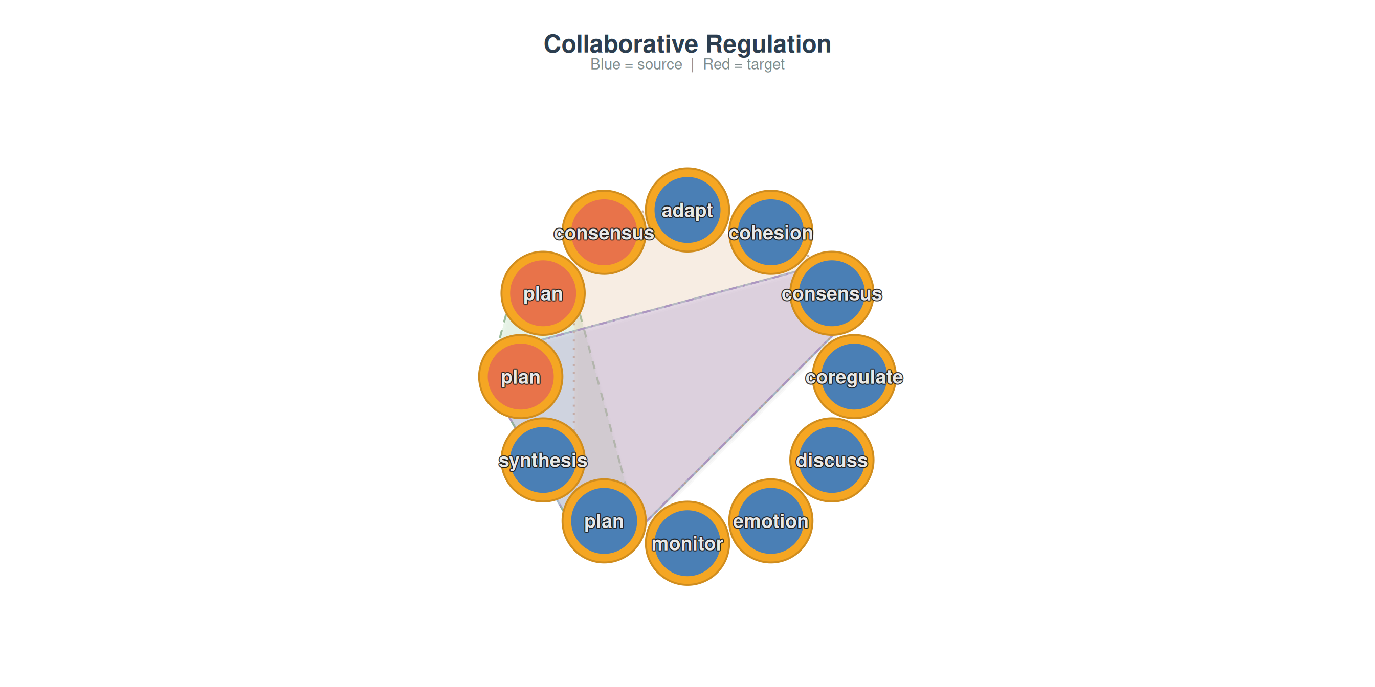

Different domains produce different higher-order signatures. Comparing these reveals whether sequential memory is a universal property of the behavioral system or specific to particular tasks.

Simplicial Complex Analysis

All the methods above analyze sequential pathways. Simplicial complex analysis takes a different perspective: it examines the topological structure of the network itself.

What is a simplicial complex?

A standard network captures pairwise relationships: node A connects to node B. But many interactions involve groups: states A, B, and C may all be densely interconnected, forming a triangle. A simplicial complex formalizes this:

A 0-simplex is a single node
A 1-simplex is an edge (two connected nodes)
A 2-simplex is a filled triangle (three mutually connected nodes)
A $k$ -simplex is a group of $k+1$ mutually connected nodes

The clique complex turns every clique into a simplex, lifting a flat graph into a multi-dimensional topological object.

Building the complex

sc <- build_simplicial(net, threshold = 0.05)
sc

Clique Complex
  9 nodes, 511 simplices, dimension 8
  Density: 100.0%  |  Mean dim: 3.51  |  Euler: 1
  f-vector: (f0=9 f1=36 f2=84 f3=126 f4=126 f5=84 f6=36 f7=9 f8=1)
  Betti: b0=1
  Nodes: Command, Correct, Frustrate, Inquire, Interrupt, Refine, Request, Specify, Verify

Topological descriptors

f-vector $(f_0, f_1, f_2, \ldots)$ : counts simplices at each dimension.
Betti numbers $(\beta_0, \beta_1, \beta_2, \ldots)$ : the central invariants. $\beta_0$ = connected components, $\beta_1$ = independent loops, $\beta_2$ = enclosed voids.
Euler characteristic $\chi = \sum (-1)^k f_k = \sum (-1)^k \beta_k$ . For a contractible complex, $\chi = 1$ .
Simplicial degree: how many higher-dimensional simplices each node participates in.

simplicial_degree(sc)

       node d0 d1 d2 d3 d4 d5 d6 d7 d8 total
1   Command  1  8 28 56 70 56 28  8  1   255
2   Correct  1  8 28 56 70 56 28  8  1   255
3 Frustrate  1  8 28 56 70 56 28  8  1   255
4   Inquire  1  8 28 56 70 56 28  8  1   255
5 Interrupt  1  8 28 56 70 56 28  8  1   255
6    Refine  1  8 28 56 70 56 28  8  1   255
7   Request  1  8 28 56 70 56 28  8  1   255
8   Specify  1  8 28 56 70 56 28  8  1   255
9    Verify  1  8 28 56 70 56 28  8  1   255

plot(sc)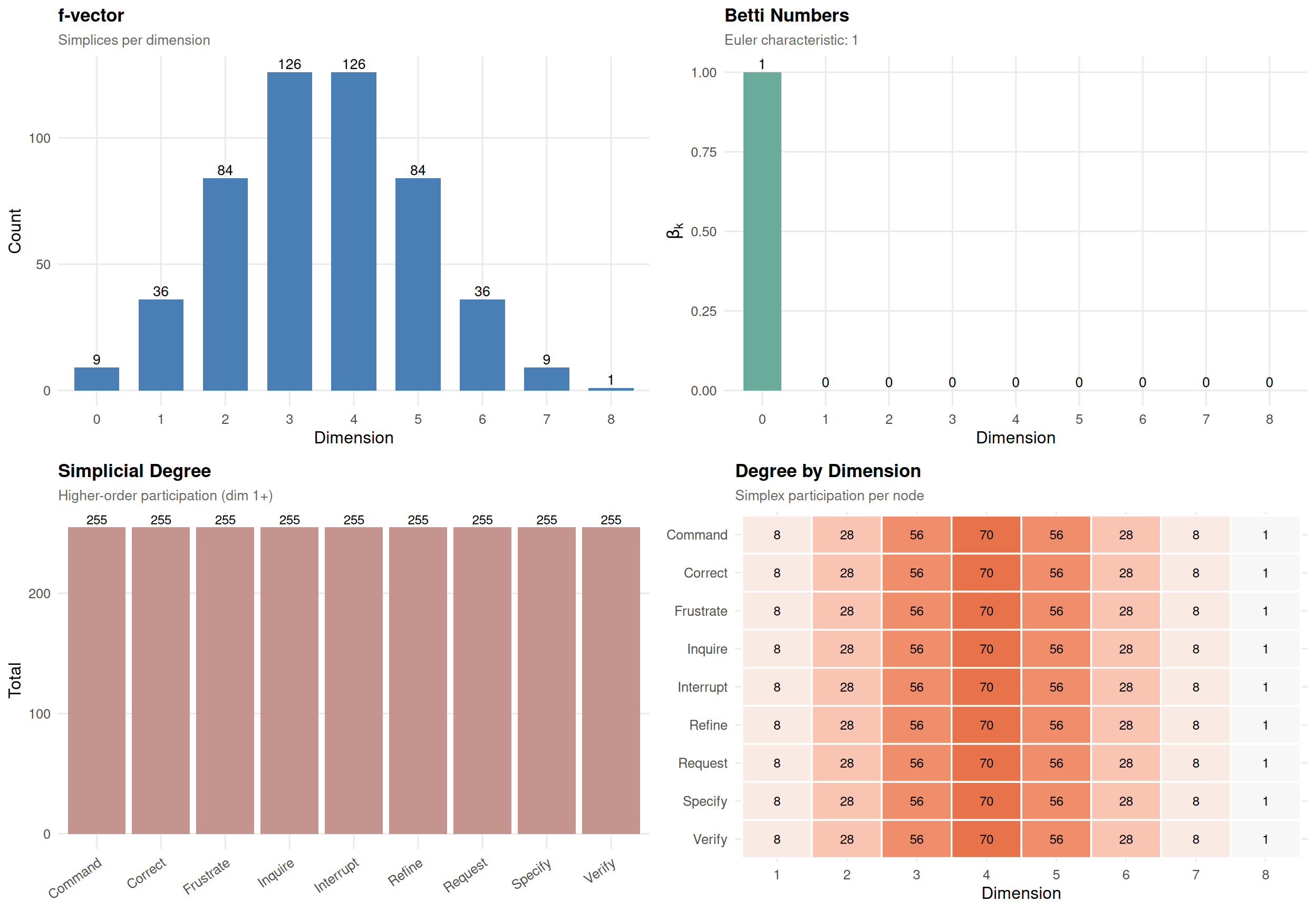

The four panels show:

f-vector (top-left): the number of simplices at each dimension. A long descending sequence with non-trivial counts at $k \geq 2$ means the network has many small densely-connected pockets, not just edges.
Betti numbers (top-right): the central topological invariants, with the Euler characteristic in the subtitle. $\beta_0$ counts disconnected components; $\beta_1$ is the number of independent loops (1-cycles that aren’t filled); $\beta_2$ counts enclosed 3D voids.
Simplicial degree (bottom-left): per-node participation in simplices of dimension $\geq 1$ . The most simplicially-active nodes are the topological hubs. This number can disagree with the pairwise-degree ranking — a node can have many edges but participate in few cliques.
Degree by dimension (bottom-right): the same participation, broken out by simplex dimension. A node that contributes mostly to high-dimensional simplices is part of densely-clustered subgroups; one whose row is concentrated at $k = 1$ has many edges but few clique-memberships.

Persistent Homology

A single complex at one threshold gives a static snapshot. Persistent homology reveals how topology evolves as we vary the threshold. Start with only the strongest edges and progressively add weaker ones. Features that persist across a wide range are topologically robust.

ph <- persistent_homology(net, n_steps = 25)
ph

Persistent Homology
  25 filtration steps [0.6197 → 0.0062]
  Features: b0: 8 (1 persistent)  |  b1: 3 (0 persistent)  |  b3: 70 (70 persistent)
  Longest-lived:
    b0: 0.6197 → 0.0000 (life: 0.6197)
    b0: 0.6197 → 0.1707 (life: 0.4491)
    b0: 0.6197 → 0.1958 (life: 0.4239)

plot(ph)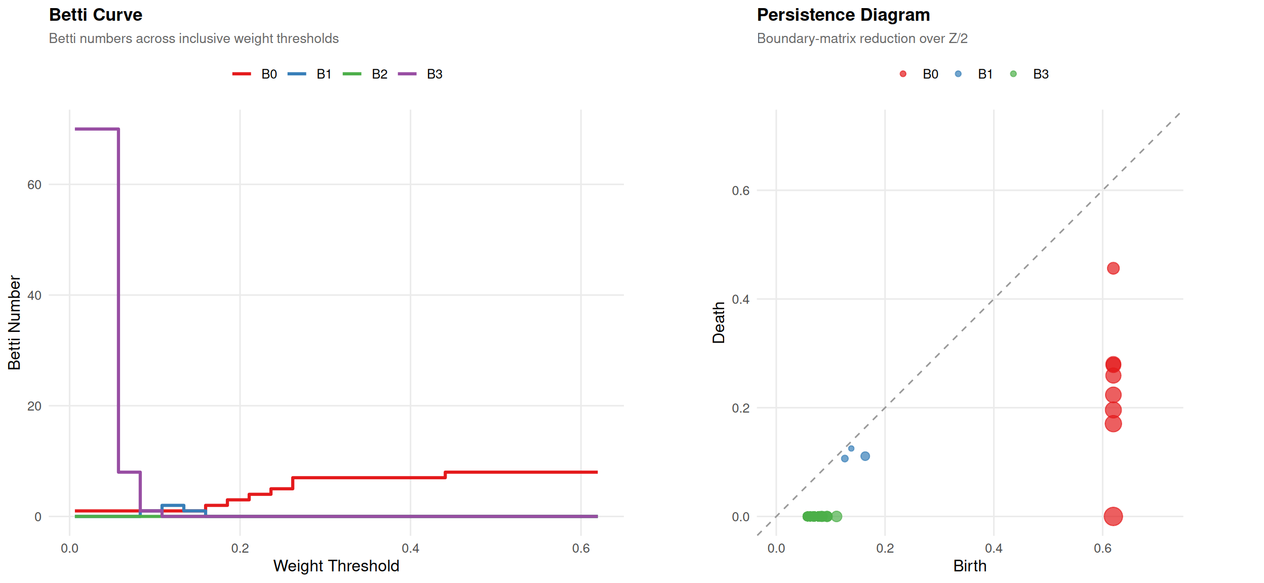

Betti curve (left) — read it as a filtration in reverse: start with only the strongest edges (high threshold = a sparse graph, many components, $\beta_0$ large) and trace what happens as the threshold drops and weaker edges are added. Components merge into one another so $\beta_0$ falls; new loops appear (so $\beta_1$ jumps up) and later get filled in by triangles (so $\beta_1$ falls again). The shape of these curves is a fingerprint of the network’s topology — a smooth monotone $\beta_0$ curve means the graph is well-connected at every scale, while a long flat plateau with sudden drops marks discrete merging events.

Persistence diagram (right): each point is one topological feature, plotted at its (birth threshold, death threshold). Points hug the diagonal when birth and death are close — those are short-lived features, almost certainly noise. Points far above the diagonal lived through a wide range of thresholds and are the robust topological signal. Color encodes dimension; size encodes persistence (death − birth) so the most persistent features pop visually.

Q-Analysis

Q-analysis (Atkin 1974) measures connectivity at multiple levels of structural sharing. Two maximal simplices are q-connected if they share a face of dimension $\geq q$ :

q = 0: share at least one node
q = 1: share at least one edge
q = 2: share at least one triangle

qa <- q_analysis(sc)
qa

Q-Analysis (max q = 8)
  Components: q8:1 q7:1 q6:1 q5:1 q4:1 q3:1 q2:1 q1:1 q0:1
  Fully connected at all q levels
  Structure: Command:8 Correct:8 Frustrate:8 Inquire:8 Interrupt:8 Refine:8 Request:8 Specify:8 Verify:8

plot(qa)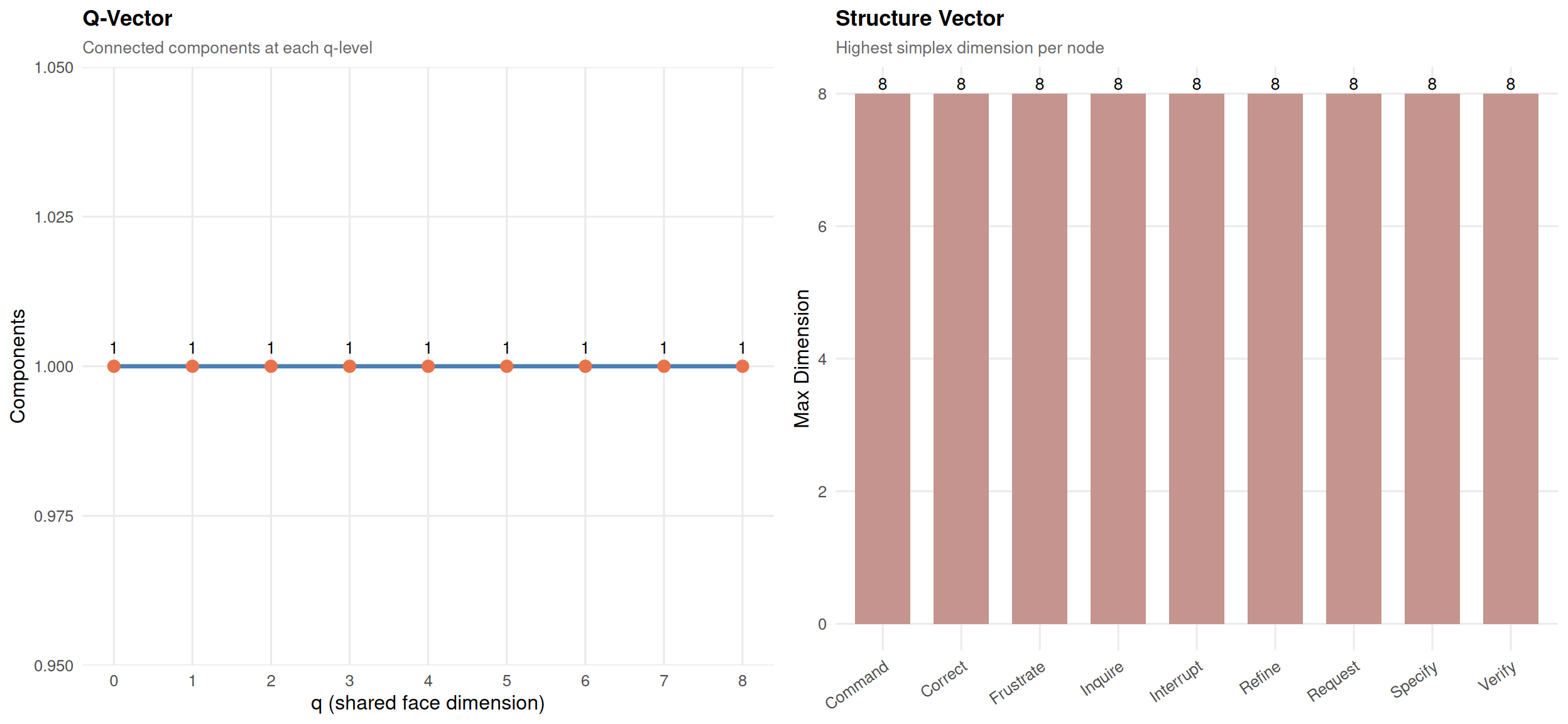

The left panel is the Q-vector: number of $q$ -connected components at each level $q$ , plotted right-to-left as $q$ decreases. Read it as a fragmentation profile of the complex.

At very high $q$ : only simplices that share a large face are linked. Most simplices stand alone, so the component count is high.
As $q$ drops: the connectivity criterion relaxes. Simplices that share even one or two vertices now count as connected, so components merge and the count falls.
At $q = 0$ : any two simplices sharing a single vertex are linked. Usually one big component.

The fragmentation point is the largest $q$ at which the count first rises above 1. Below it the complex hangs together as one piece through high-order shared structure (groups of simplices that overlap in big faces). Above it that high-order glue is broken — sub-structures become isolated islands held together only by sparse low-order overlaps. A high fragmentation point means strong cohesion: many simplices share substantial substructure. A low one means simplices are stitched together mostly through one or two shared vertices, with no deep shared structure.

The right panel shows the structure vector: the maximum simplex dimension each node participates in, sorted descending. Nodes at the top are members of the densest clique-groups in the network.

Pathway Complex from HON

An alternative to the clique complex: build a simplicial complex from the pathways discovered by HON — topology derived from sequential dynamics rather than network structure:

sc_hon <- build_simplicial(hon, type = "pathway", max_pathways = 30)
sc_hon

Pathway Complex
  9 nodes, 31 simplices, dimension 3
  Density: 12.2%  |  Mean dim: 1.00  |  Euler: 1
  f-vector: (f0=9 f1=14 f2=7 f3=1)
  Betti: b0=2 b1=1
  Nodes: Command, Correct, Frustrate, Inquire, Interrupt, Refine, Request, Specify, Verify

plot(sc_hon)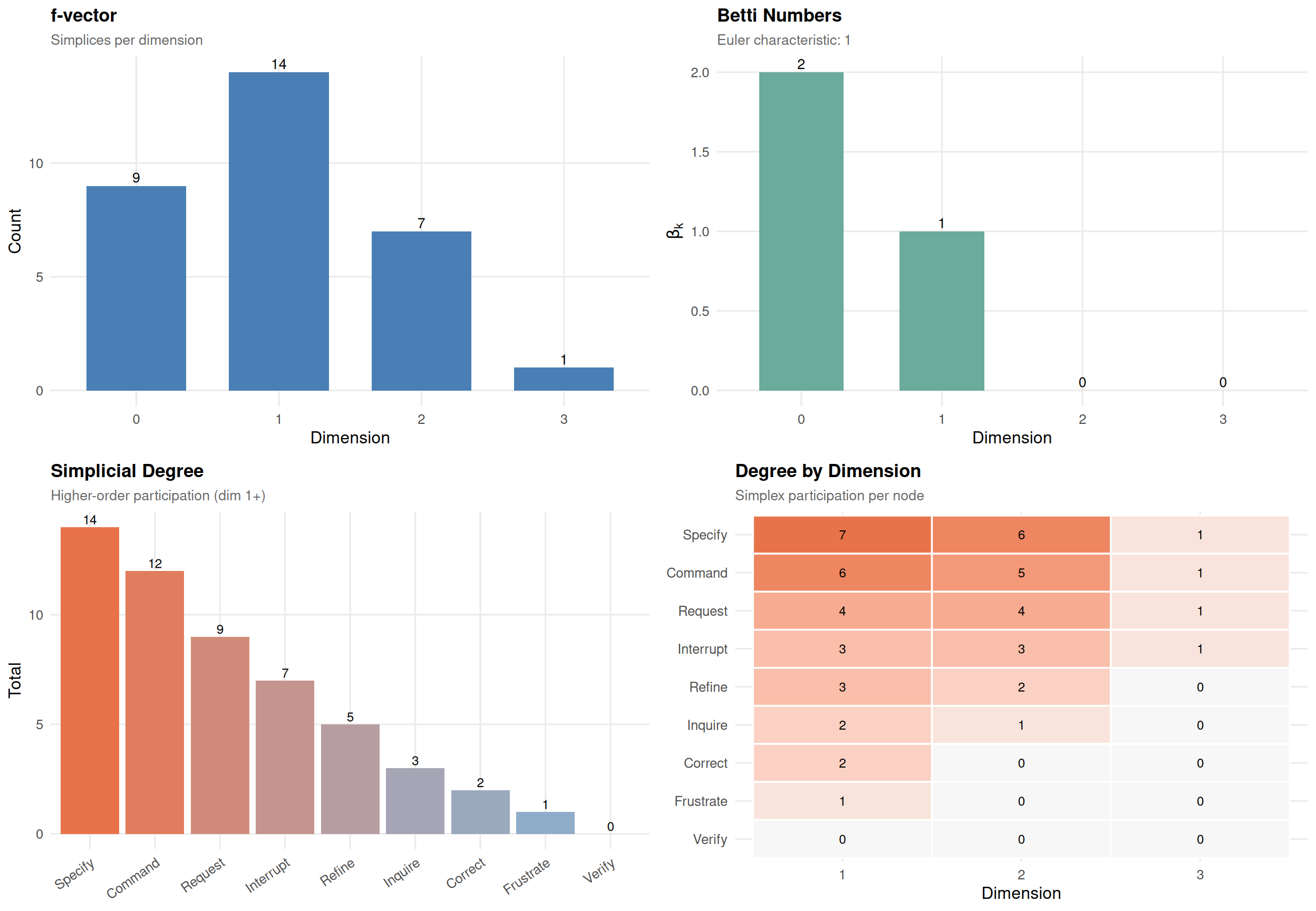

In the pathway complex, each higher-order pathway becomes a simplex. $\beta_0 > 1$ means some states are sequentially disconnected. $\beta_1 > 0$ means there are cyclic pathway structures.

Verification

All simplicial computations are cross-validated against igraph’s clique-finding and verified via the Euler-Poincaré theorem:

verify_simplicial(net$weights, threshold = 0.05)

  Cliques:  MATCH (511 simplices)
  Betti:    b0=1 b1=0 b2=0 b3=0 b4=0 b5=0 b6=0 b7=0 b8=0
  Euler:    1 (Euler-Poincare: VERIFIED)

Summary

Step	Method	Function	What it reveals
1	TNA	`build_network()`	First-order transition structure
2	MOGen	`build_mogen()`	Whether higher-order is needed (information criteria)
3	Markov order test	`markov_order_test()`	Whether higher-order is needed (permutation-exact LRT)
4	Transition entropy	`transition_entropy()`	Per-state predictability and chain entropy rate
5	HON	`build_hon()`	Where sequential context changes transitions
6	HYPA	`build_hypa()`	Which paths are anomalously frequent or rare
7	Visualization	`plot_simplicial()`	Blob diagrams of pathways (also accepts `mogen_transitions()` data.frames)
8	Simplicial	`build_simplicial()`	Topological structure
9	Persistence	`persistent_homology()`	Robustness across scales
10	Q-analysis	`q_analysis()`	Multi-level connectivity

The key progression:

TNA answers: what transitions exist?
MOGen + Markov order test answer: is first-order enough? (and disagree informatively when BIC is conservative)
Transition entropy answers: which states are unpredictable hubs vs. deterministic gateways?
HON answers: where does context matter?
HYPA answers: which sequences are surprisingly frequent — or surprisingly avoided?
Simplicial analysis answers: what is the shape of the interaction space?

References

Atkin, R. H. (1974). Mathematical Structure in Human Affairs. Heinemann Educational.
Battiston, F., et al. (2020). Networks beyond pairwise interactions: Structure and dynamics. Physics Reports, 874, 1–92.
LaRock, T., Scholtes, I., & Eliassi-Rad, T. (2020). HYPA: Efficient detection of path anomalies in time series data on networks. EPJ Data Science, 9(1), 15.
Scholtes, I. (2017). When is a network a network? Multi-order graphical model selection in pathways and temporal networks. Proceedings of the 23rd ACM SIGKDD International Conference on Knowledge Discovery and Data Mining, 1037–1046.
Xu, J., Wickramarathne, T. L., & Chawla, N. V. (2016). Representing higher-order dependencies in networks. Science Advances, 2(5), e1600028.