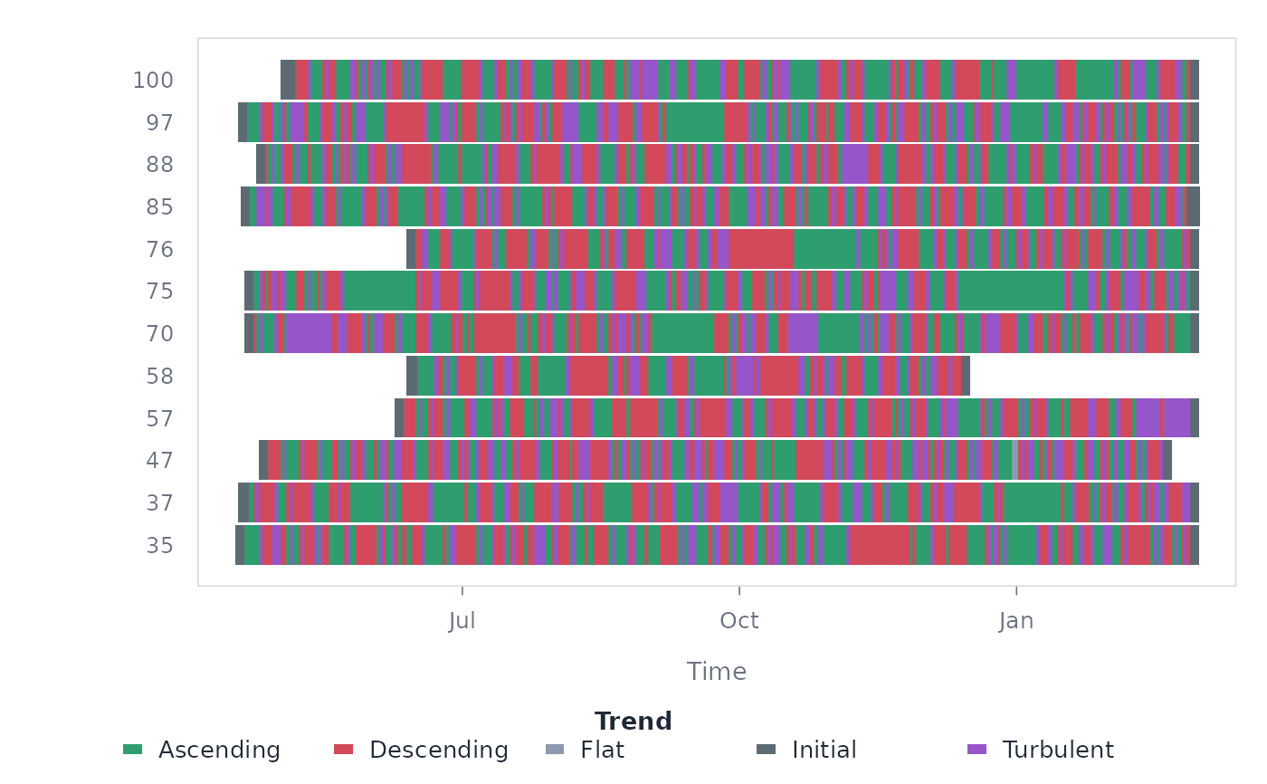
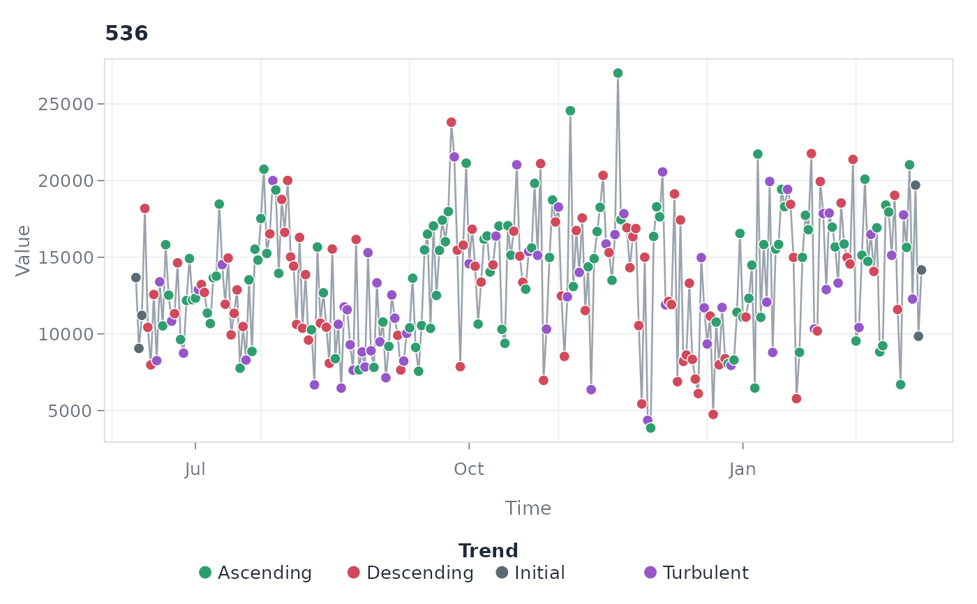
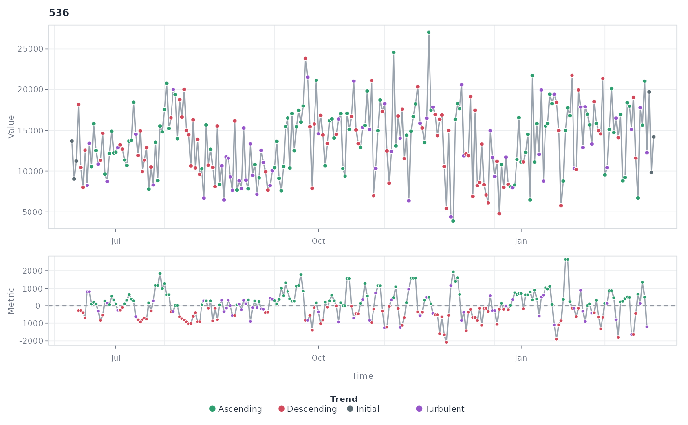
Plot a trend classification — plot.tsn

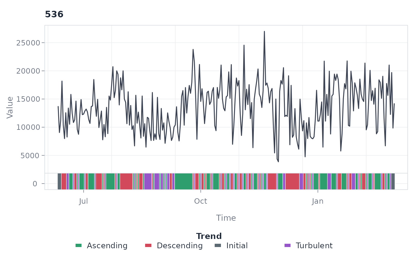
Four views of a trend classification, selected with type. "points" (default) draws each series with observations coloured by trend state; "ribbon" runs the trend classification as a strip underneath the clean series line; "heatmap" draws one row per series with one coloured tile per observation, comparing trend timing across many series; "panels" stacks each series above its rolling trend metric (the slope or correlation trend() classified on) so a state change can be read against the metric that produced it.

Usage

# S3 method for class 'tsn_trend'
plot(
  x,
  type = c("points", "ribbon", "heatmap", "panels"),
  series = NULL,
  max_series = NULL,
  columns = NULL,
  palette = NULL,
  line_color = "#9AA3AD",
  line_width = 1.3,
  point_size = 1.05,
  strip_height = 0.1,
  sort = "none",
  border = FALSE,
  flat_band = TRUE,
  legend = TRUE,
  xlab = "Time",
  ylab = "Value",
  cex = 1,
  grid = TRUE,
  background = "#FFFFFF",
  ...
)

Arguments

x: A tsn_trend result.
type: The view: "points", "ribbon", "heatmap", or "panels".
series: Optional character vector of series IDs to display.
max_series: Maximum number of series to draw (25 for the heatmap, 4 for the panel view, 10 otherwise).
columns: Number of panel columns.
palette: Optional named colours overriding individual trend states (e.g. c(Ascending = "forestgreen")).
line_color: Series line colour.
line_width: Series line width.
point_size: Observation point size.
strip_height: Ribbon strip height as a fraction of the panel.
sort: Heatmap row order: "none", "mean", or "state".
border: Whether heatmap tiles carry a thin separator border.
flat_band: For type = "panels", shade the epsilon flat band on the metric panel so the classification threshold is visible.
legend: Whether to draw the legend row.
xlab, ylab: Axis titles.
cex: Global text size multiplier.
grid: Whether to draw the background grid.
background: Panel background colour.
...: Reserved for future options.

Value

x, invisibly.

Examples

data(steps)
complete <- subset(steps, !is.na(steps))
classified <- trend(
  complete,
  value = "steps", id = "id", time = "day", window = 7
)
plot(classified, series = "536")

plot(classified, "ribbon", series = "536")

plot(classified, "panels", series = "536")

plot(classified, "heatmap", max_series = 12)