Constructing Time Series Networks

Introduction

Time series analysis traditionally represents temporal data as observations indexed by time, with attention directed to quantities such as level, variation, dependence, and change. A network representation offers a complementary view: it replaces, or augments, the explicit time index with a relational structure in which nodes stand for observations, temporal states, or local windows, and edges encode a defined relationship between them. That relationship may be geometric visibility, numerical similarity, a state transition, a co-occurrence, or a weighted dependence. A time series therefore does not have a single canonical network. The network that results is determined jointly by the chosen representation and by the structural question that representation is designed to answer.

The tsn package provides a set of these representations while keeping the modelling choices explicit at every step. discretize() maps continuous observations onto a finite set of ordered states and so yields a symbolic version of the series. trend() characterizes local direction and separates short-range increase, decrease, stability, and turbulence. vg() constructs a visibility graph, in which observations are joined when the geometry of the series makes them mutually visible. tsn() is the general distance-network constructor over complete series, local windows, or individual observations; this vignette applies it to overlapping windows joined by their similarity.

Once a series has been reduced to a sequence of states, its dynamics can be examined through transition network analysis. ts_tna() builds a transition network whose edges carry conditional transition probabilities. ts_ftna() builds the corresponding frequency network, ts_cna() a co-occurrence network, and ts_atna() an attention-weighted transition network. These four constructions summarize different properties of the same symbolic sequence and are complementary rather than interchangeable. Finally, series_networks() extracts and indexes the network model attached to each source series, retaining the model type, the shared state alphabet, and the provenance needed to trace a network back to its data.

Every representation in this vignette is developed on one fixed segment of one measured variable, so that the constructions can be compared without any change in the underlying data. Network figures are produced by the package’s plot() methods through cograph, and the four transition-network constructors require the Nestimate package; both are optional and used only where noted.

Scientific question	Function	Result	What it captures
How can a continuous series be represented as a sequence of discrete states?	`discretize()`	Tidy state table	Maps continuous observations onto a finite, ordered state alphabet, making recurring levels and ranges explicit.
How does the series change locally over time?	`trend()`	Tidy trend table	Labels each observation by its local direction: increase, decrease, stability, or turbulence.
Which observations are connected by geometric visibility?	`vg()`	Visibility network	Connects observations that can “see” each other over the intervening values.
Which time windows are similar in value or shape?	`tsn()`	Distance network	Relates local windows by their proximity, exposing repeated or structurally similar segments.
How likely is one state to be followed by another?	`ts_tna()`	Transition network (TNA)	Weights directed edges by the conditional probability of each successive transition.
How often does the series move from one state to another?	`ts_ftna()`	Frequency network (FTNA)	Weights directed edges by the observed count of each successive transition.
Which states co-occur within the sequence?	`ts_cna()`	Co-occurrence network (CNA)	Uses undirected edges to represent state co-occurrence, ignoring direction.
Which transitions receive the greatest attention weight?	`ts_atna()`	Attention-weighted network (ATNA)	Weights directed edges by model-assigned attention rather than raw counts.
How is each network associated with its source series?	`series_networks()`	Indexed model collection	Organizes extracted models by source series while preserving their correspondence and provenance.

In short, discretize() defines the states, trend() describes local direction, vg() describes geometric visibility, and tsn() describes similarity between temporal windows. The ts_tna() family then builds transition networks from the state sequence, differing only in the quantity assigned to their edges, and series_networks() indexes the results by source series.

Data

The motivation data set bundled with the package is an example of experience-sampling, or intensive longitudinal, data: the same respondent was prompted several times a day and asked to report, in the moment, how they felt about the activity they were engaged in. Each of its 4,871 rows is one such momentary report, collected between September 2018 and July 2021, and no values are missing. The thirteen columns fall into a few natural groups. Three record motivation (autonomy, competence, relatedness); three record appraisal of the current activity (pleasure, interest, importance); several describe the situation and its emotional framing, together with a categorical context label whose values are Home, Work, Personal, and Other; and one records overall mood. Two further columns place each report in time, giving the calendar date and the position of the report within that day’s sequence of prompts.

This vignette follows a single one of these signals, the pleasure rating, which captures how pleasant the respondent found the current activity at the moment of the prompt. To keep every network small enough to read in full, the analysis uses only the first 60 reports, which each verb selects by name from the data frame. Passing the data frame rather than a bare vector preserves the recorded order of the observations, and that order is what every method below treats as the flow of time.

data("motivation", package = "tsn")

pleasure <- head(motivation, 60)

dim(pleasure)
#> [1] 60 13

These 60 reports were collected over 21 days, from 29 September to 19 October 2018. The pleasure ratings occupy the observed range 6 to 44, with a median of 30, a mean of 26.8, and a standard deviation of about 10, so they spread across a wide band rather than clustering near a single value. The segment carries no systematic trend: the first twenty reports average 27.5 and the last twenty average 27.0, essentially unchanged. The representations that follow should therefore be read as descriptions of short-run fluctuation around a roughly constant level, not of a rising or falling series. The distinction matters for interpretation, because several of the constructions below, in particular the visibility graph and the trend labels, respond to the local rises and falls of the series rather than to its overall direction.

Transition Network Analysis

Transition Network Analysis starts by turning the observed series into a finite sequence of states. The aim is not to discard the measured values but to obtain a symbolic representation in which dynamics can be studied as movement among a fixed set of states. discretize() performs this step, assigning each observation to one state and returning one tidy row per observation.

Here the default quantile discretization splits the values into three empirical groups, labelled Low, Middle, and High. The resulting sequence keeps the temporal order of the observations and replaces their continuous values with ordered categorical states.

states <- discretize(
  data = pleasure,
  series = "pleasure",
  labels = c("Low", "Middle", "High")
)

states
#> <tsn_states> quantile discretization (transform: none): 60 observations, 3 states
#>        id time value  state probability
#>  pleasure    1    32 Middle           1
#>  pleasure    2    32 Middle           1
#>  pleasure    3    32 Middle           1
#>  pleasure    4    26 Middle           1
#>  pleasure    5    16    Low           1
#>  pleasure    6     6    Low           1
#>  pleasure    7    30 Middle           1
#>  pleasure    8     6    Low           1
#>  pleasure    9    44   High           1
#>  pleasure   10    42   High           1
summary(states)
#>    state count proportion mean_value
#> 1    Low    20  0.3333333   14.75000
#> 2 Middle    23  0.3833333   29.13043
#> 3   High    17  0.2833333   37.82353

Each row records the source identifier, the time index, the observed value, the assigned state, and an assignment probability. The probability column reports the confidence of the assignment: it equals 1 for a hard partition such as the quantile rule used here, and takes values in the unit interval for probabilistic discretizers such as gaussian or kde. Because the state labels follow the ordering of the values, Low, Middle, and High retain a strict ordinal meaning. Quantile boundaries do not, in general, divide the observations into exactly equal groups when values are tied; in this segment the counts are 20 Low, 23 Middle, and 17 High.

The state sequence is the intermediate object from which every transition network below is built. Its three states become the network nodes, and each adjacent pair of observations defines one possible state-to-state transition. The four constructors that follow all read this same sequence; what differs between them is the quantity placed on the edges.

plot(states, type = "ribbon")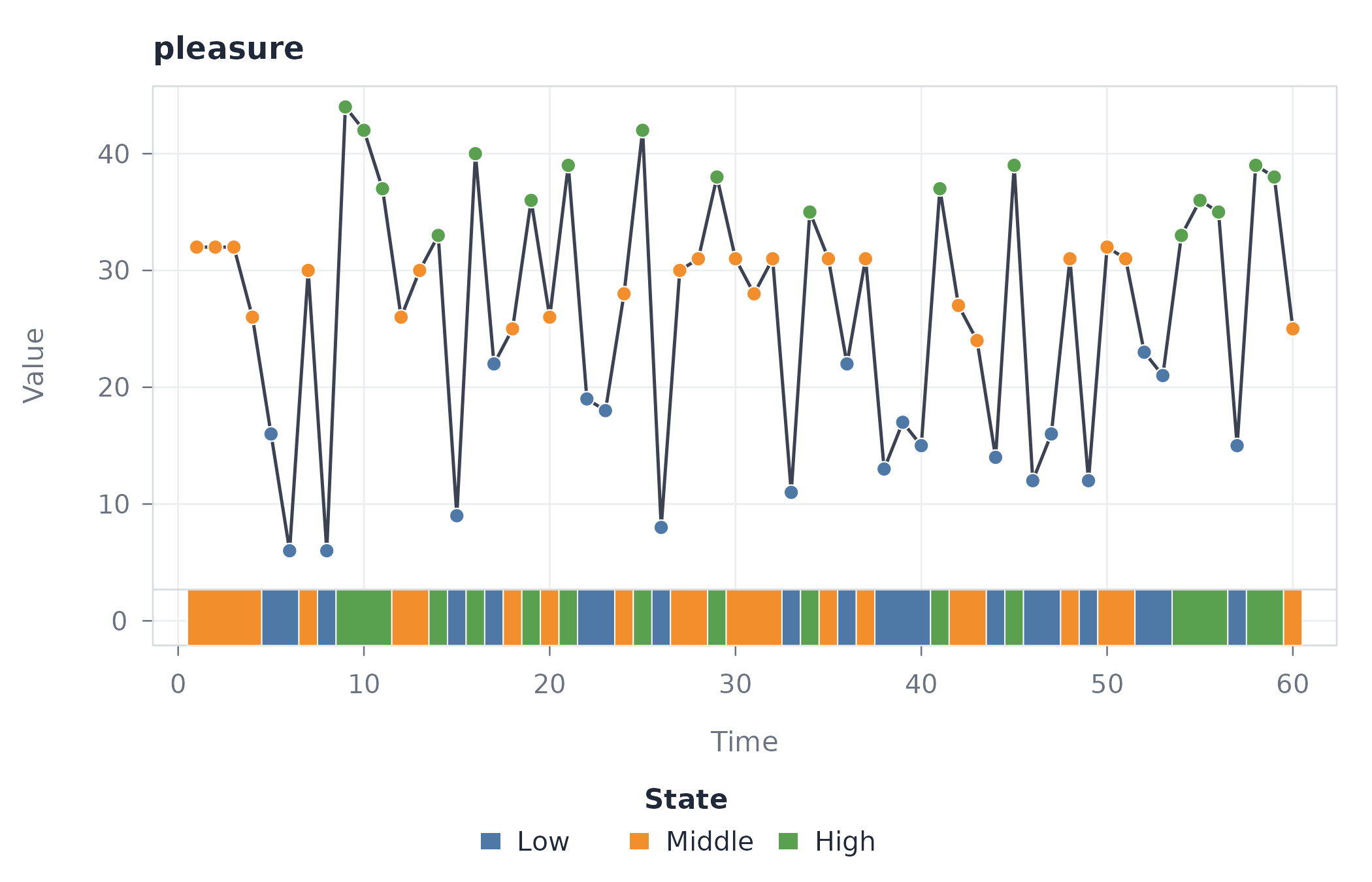

Ribbon plot of the pleasure series with a strip of Low, Middle, and High states drawn beneath the measured values along observation order.

The ribbon view places the discrete states beneath the measured series, so the correspondence between an observation and its assigned state stays visible without a full-panel overlay obscuring the values themselves.

Transition probabilities with `ts_tna()`

ts_tna() builds a directed network in which an edge runs from the current state to the next, weighted by the conditional probability of that transition. Each row of the weight matrix is a probability distribution over the possible next states, so the outgoing weights of a state sum to one.

probabilities <- ts_tna(states)

probabilities
#> Transition Network (relative probabilities) [directed]
#>   Weights: [0.227, 0.409]  |  mean: 0.333
#> 
#>   Weight matrix:
#>            Low Middle  High
#>   Low    0.300  0.350 0.350
#>   Middle 0.364  0.409 0.227
#>   High   0.353  0.353 0.294 
#> 
#>   Initial probabilities:
#>   Middle        1.000  ████████████████████████████████████████
#>   Low           0.000  
#>   High          0.000

The diagonal entries measure persistence, the probability that the next observation stays in the current state: 0.300 for Low, 0.409 for Middle, and 0.294 for High. Comparing these with the marginal state proportions (0.333, 0.383, and 0.283) separates persistence from mere prevalence. Middle and High both persist above their marginal share, so a Middle or High observation is more likely to be followed by its own state than random ordering would imply. Low sits marginally below its share (0.300 against 0.333), indicating no such tendency to persist over this short segment.

plot(probabilities)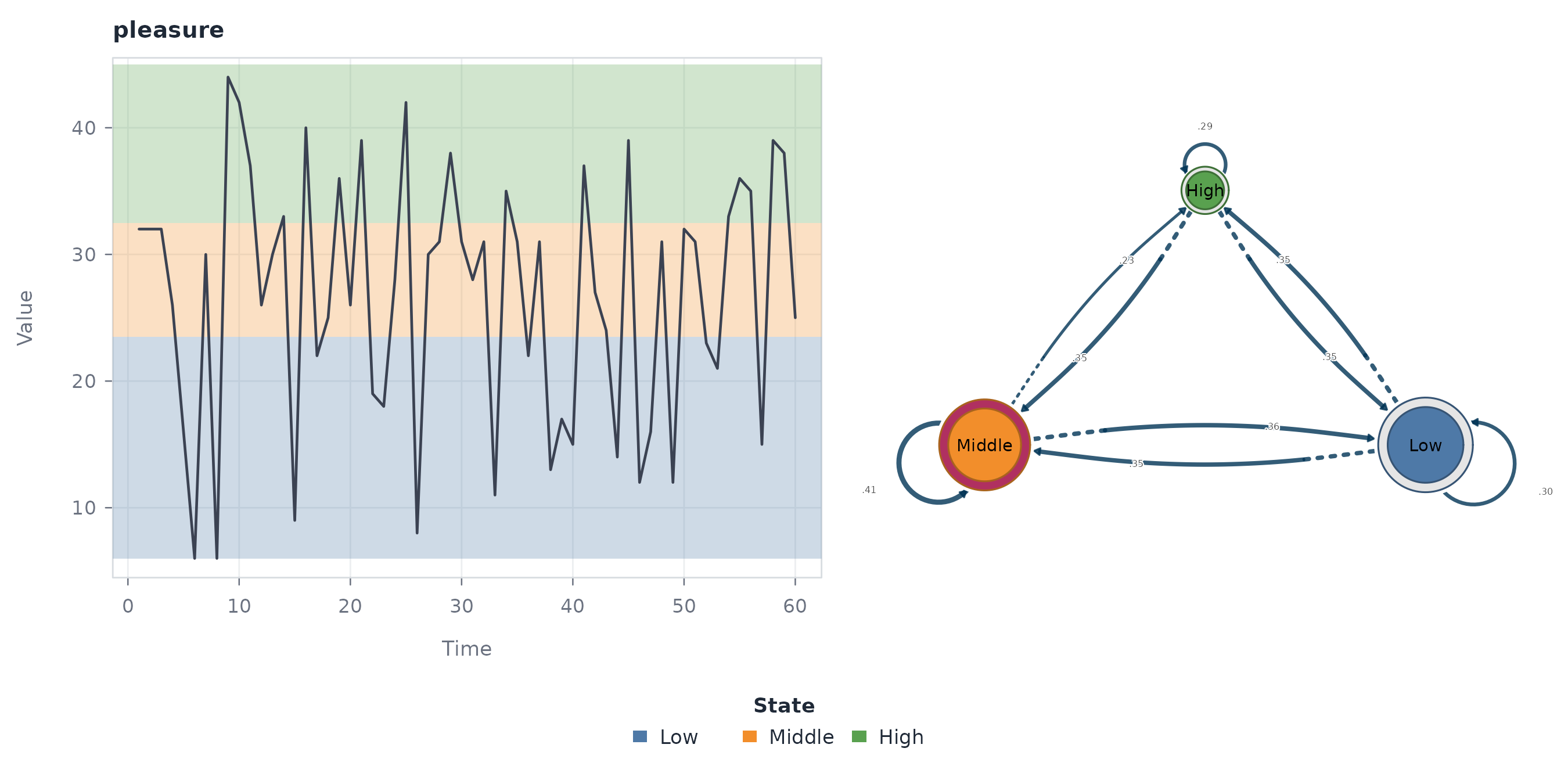

Directed transition-probability network over the Low, Middle, and High states, with arrows labelled by conditional probabilities.

Row normalization is what makes this representation interpretable. Each row is the conditional distribution of the next state given the current one, so the outgoing patterns of different states remain comparable even though the states have different marginal frequencies. A sequence of 60 observations is thereby reduced to three nodes and the directed relationships among them, with the temporal order retained as the basis for the estimates.

Transition frequencies with `ts_ftna()`

ts_ftna() weights each directed edge by the observed count of the corresponding transition, without the row normalization applied by ts_tna(). The network therefore preserves the absolute number of times each transition occurred.

counts <- ts_ftna(states)

counts
#> Transition Network (frequency counts) [directed]
#>   Weights: [5.000, 9.000]  |  mean: 6.556
#> 
#>   Weight matrix:
#>          Low Middle High
#>   Low      6      7    7
#>   Middle   8      9    5
#>   High     6      6    5 
#> 
#>   Initial probabilities:
#>   Middle        1.000  ████████████████████████████████████████
#>   Low           0.000  
#>   High          0.000

The 60 observations form 59 adjacent pairs, so the count matrix sums to 59. The most frequent single transition is Middle to Middle, which occurs 9 times and is the only self-transition that is also the largest count in its row. The Low and High rows are more evenly spread: a Low observation is followed equally often by Middle or High (7 each) rather than by another Low (6), so persistence, although present, does not dominate the raw counts here. The frequency and probability networks describe the same transitions but answer different questions: the frequency network reports how often each transition occurred, whereas the probability network reports how likely it is given the current state.

plot(counts)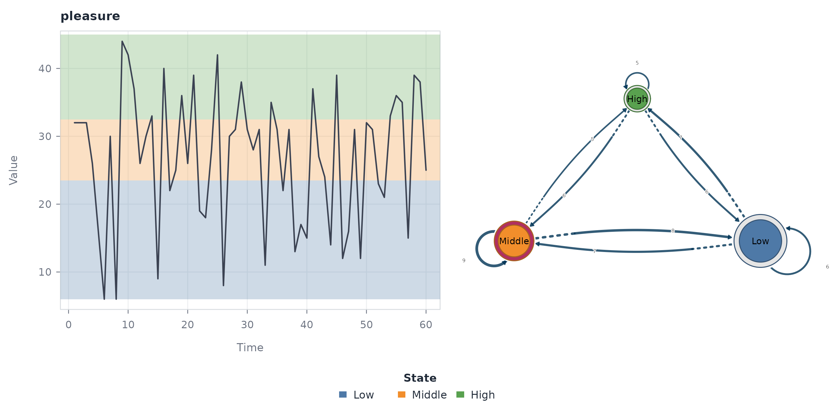

Directed frequency transition network over the three states, with arrows labelled by observed transition counts.

State co-occurrence with `ts_cna()`

ts_cna() builds an undirected, symmetric network whose edges measure how strongly two states occur together, without regard to the order in which they appear. It answers a different question from the directed transition networks.

cooccurrence <- ts_cna(states)

cooccurrence
#> Co-occurrence Network [undirected]
#>   Weights: [136.000, 460.000]  |  mean: 295.000
#> 
#>   Weight matrix:
#>          Low Middle High
#>   Low    190    460  340
#>   Middle 460    253  391
#>   High   340    391  136

For a single sequence, these co-occurrence counts follow directly from the marginal state frequencies. An off-diagonal entry is the product of the two state counts, so the Low-Middle weight is 20 * 23 = 460; a diagonal entry counts the unordered pairs within a state, so the Low-Low weight is 20 * 19 / 2 = 190. The network therefore reflects the composition of the state alphabet rather than the temporal direction of transitions. A strong edge means the two states are both common, not that one tends to follow the other.

plot(cooccurrence)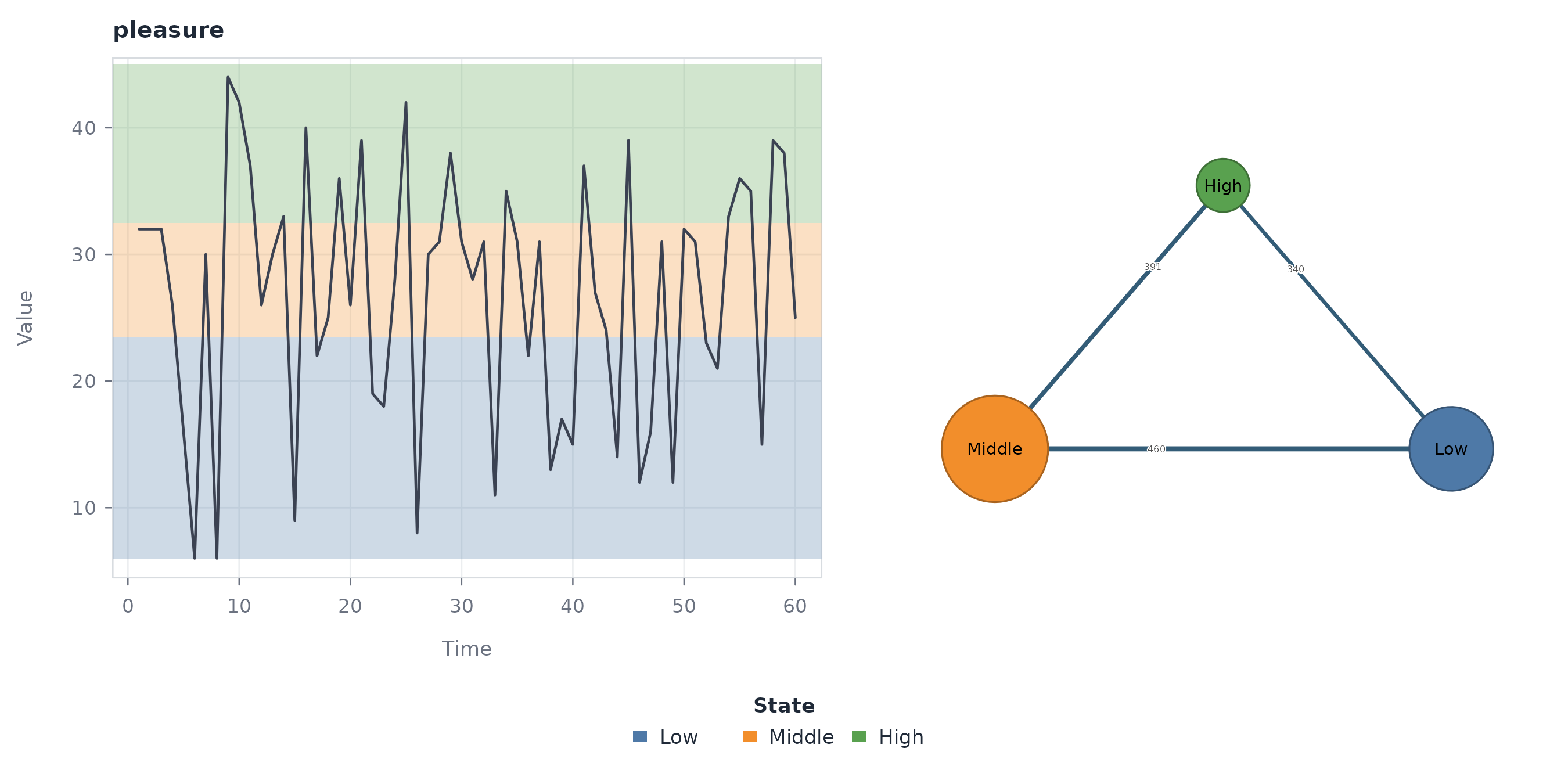

Undirected co-occurrence network over the three states, with symmetric edges weighted by state co-occurrence.

The symmetric drawing makes the distinction explicit: an edge carries no source-to-target direction, in contrast to the transition networks above.

Attention-weighted transitions with `ts_atna()`

ts_atna() assigns each transition an attention weight rather than a count or a probability. The edge weights are accumulated attention values and are not on the scale of either the frequency or the probability network.

attention <- ts_atna(states)

attention
#> Attention Network (decay-weighted transitions) [directed]
#>   Weights: [2.875, 5.015]  |  mean: 3.778
#> 
#>   Weight matrix:
#>            Low Middle  High
#>   Low    3.524  4.055 4.031
#>   Middle 5.015  4.801 2.988
#>   High   3.085  3.625 2.875 
#> 
#>   Initial probabilities:
#>   Middle        1.000  ████████████████████████████████████████
#>   Low           0.000  
#>   High          0.000

The weights range from 2.875 to 5.015. Unlike the frequency and probability networks, the largest weights here are off-diagonal: the strongest attention-weighted transition is Middle to Low (5.015), and the persistence diagonals are not the dominant entries in their rows. The attention mechanism consequently redistributes emphasis away from the self-transitions that the raw counts favour, and the weights should be read on the model’s own attention scale rather than compared directly with counts or probabilities.

plot(attention)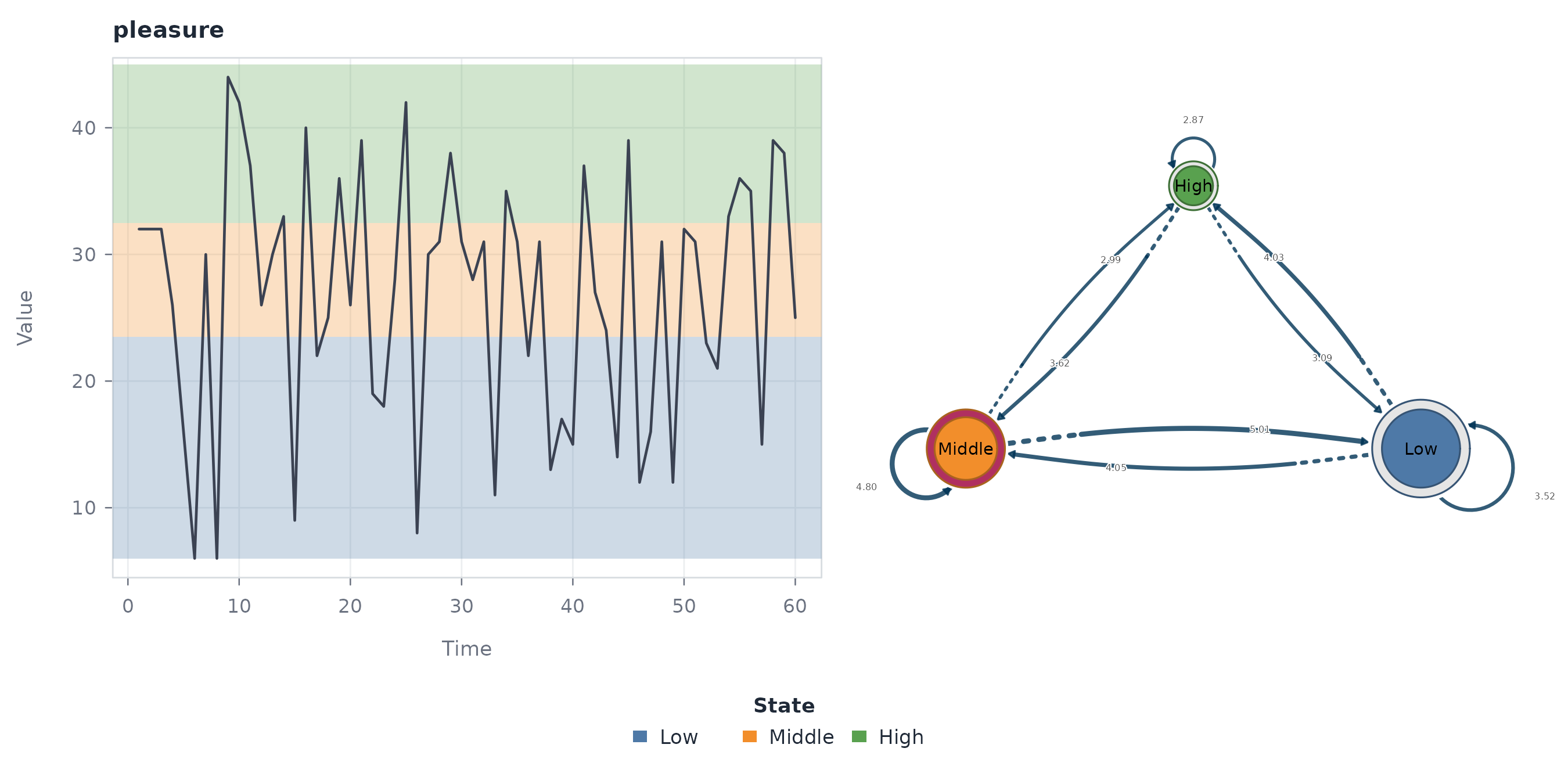

Directed attention-weighted transition network over the three states, with edges weighted by accumulated attention values.

Indexing the model with `series_networks()`

series_networks() returns an indexed collection of the network models attached to the source series. It is designed for analyses that extract networks across many series at once, where the index preserves the link between each series and its model. With a single input series it returns one entry, corresponding to pleasure.

individual <- series_networks(probabilities)

individual
#>    series type observations states edges
#>  pleasure  tna           60      3     9

The index records the source series, the network type, and the number of observations, states, and edges. For the transition-probability network the three states generate nine directed relationships, the six between distinct states plus the three self-transitions.

plot(individual)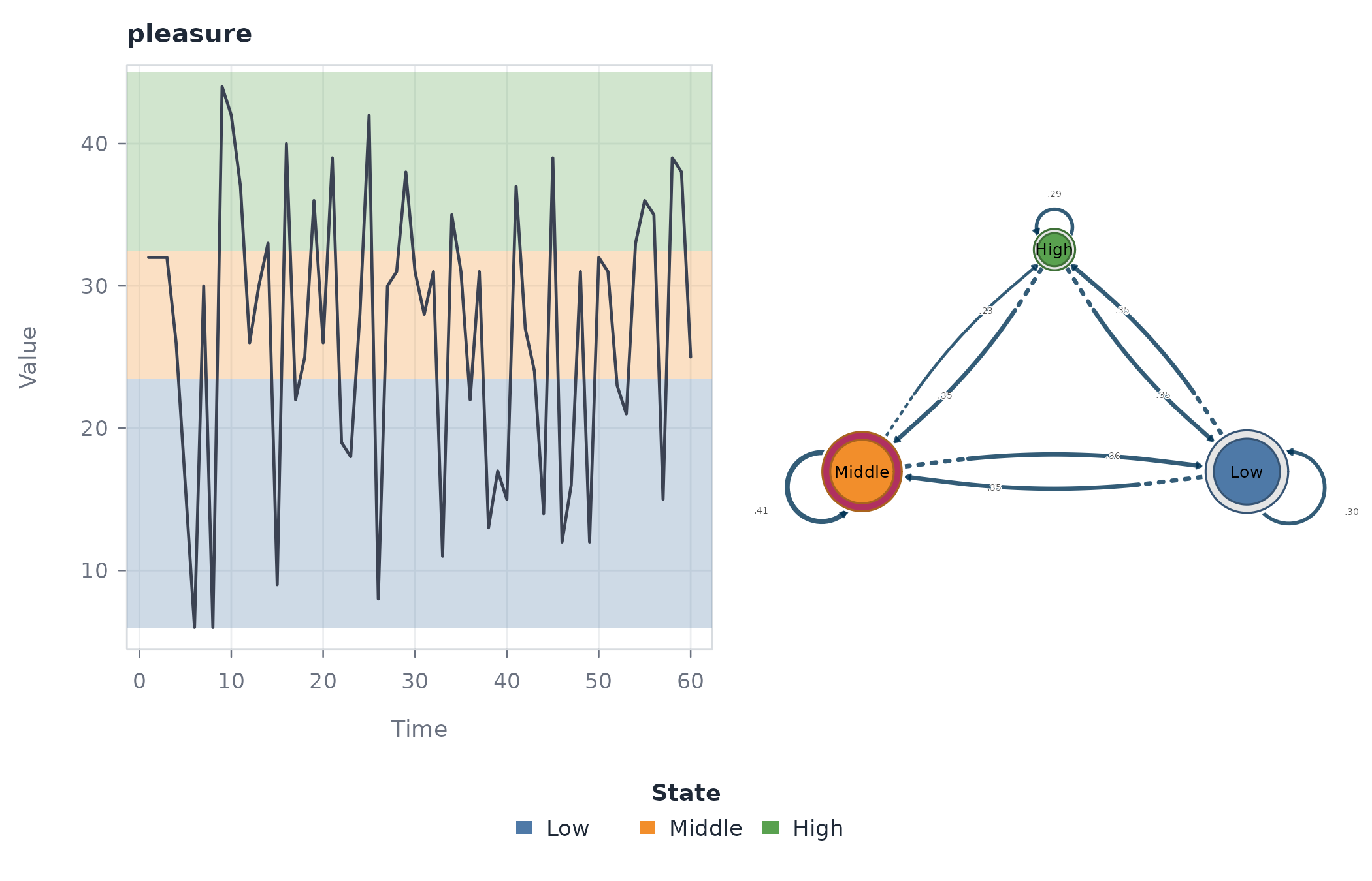

The single indexed transition-probability network for the pleasure series, drawn from the series_networks collection.

The collection thus provides a higher-level handle on the extracted networks while keeping their provenance. Given several source series, the same structure organizes and compares their models systematically.

Local direction with `trend()`

trend() estimates a rolling local slope and labels each observation as Ascending, Descending, Flat, Turbulent, Missing Data, or Initial. The window is adaptive and defaults to one tenth of the series length, which is 6 observations here, and the default Theil-Sen slope limits the influence of isolated extreme ratings.

directions <- trend(
  data = pleasure,
  series = "pleasure"
)

directions
#> <tsn_trend> slope (robust), window 6: 60 observations across 1 series
#>        id time value    metric      state
#>  pleasure    1    32        NA    Initial
#>  pleasure    2    32        NA    Initial
#>  pleasure    3    32 -5.333333 Descending
#>  pleasure    4    26 -5.333333 Descending
#>  pleasure    5    16 -5.200000 Descending
#>  pleasure    6     6  1.333333  Ascending
#>  pleasure    7    30  7.000000  Turbulent
#>  pleasure    8     6  6.200000  Ascending
#>  pleasure    9    44 -0.800000 Descending
#>  pleasure   10    42 -3.500000  Turbulent
summary(directions)
#>        state count proportion
#> 1  Ascending    21 0.35000000
#> 2 Descending    17 0.28333333
#> 3       Flat     4 0.06666667
#> 4  Turbulent    13 0.21666667
#> 5    Initial     5 0.08333333

Ascending is the most common label with 21 observations, followed by Descending with 17, Turbulent with 13, Initial with 5, and Flat with 4. The near balance between ascending and descending positions is what a segment without drift should produce: local direction keeps reversing rather than accumulating in one direction. Initial marks the leading positions that lack a complete centered window, and Missing Data would mark absent values, of which this segment has none.

plot(directions)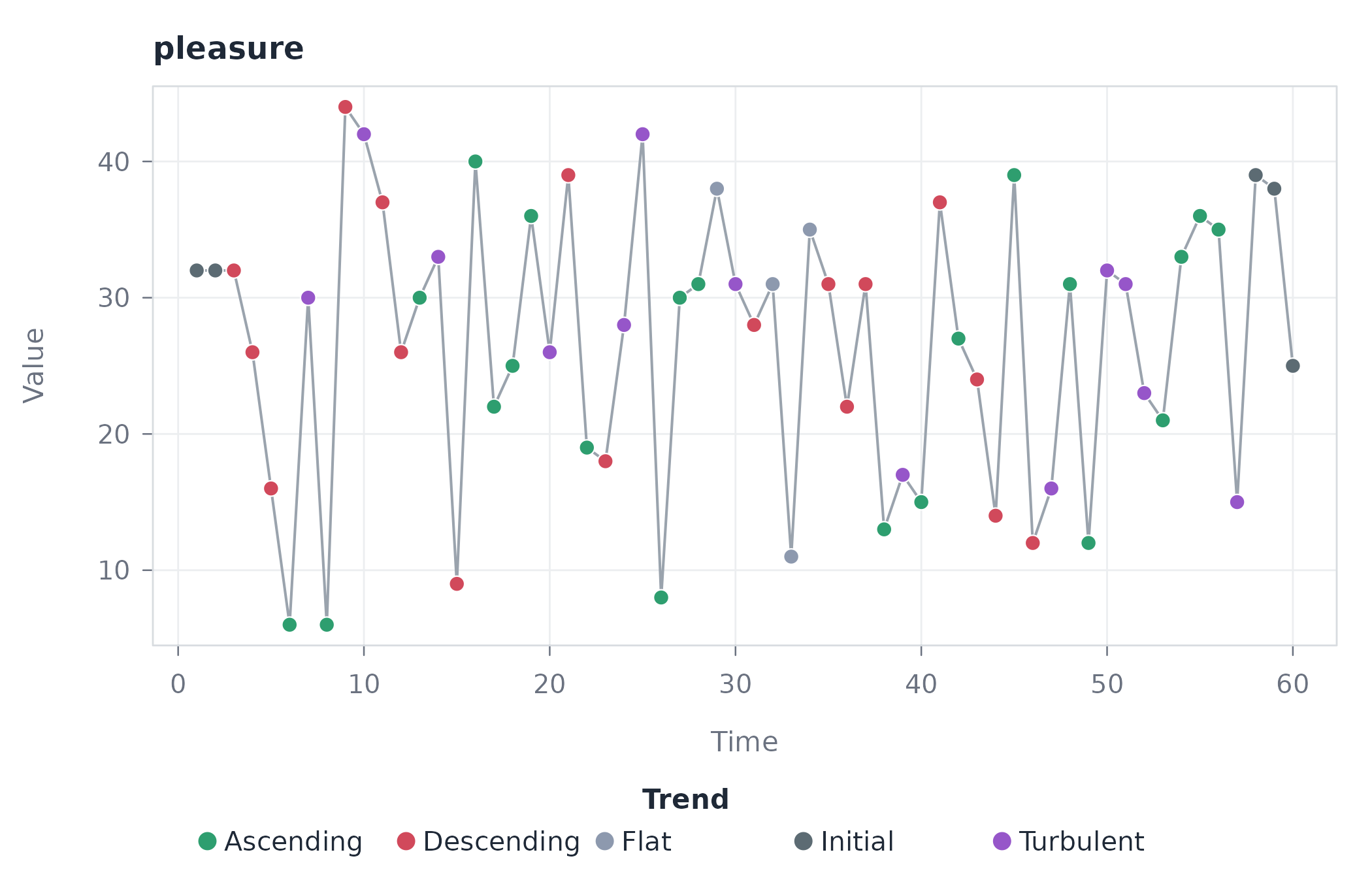

The pleasure series with each observation coloured by its trend label: Ascending, Descending, Flat, Turbulent, or Initial.

The default plot colours each observation by its trend label.

plot(directions, type = "panels")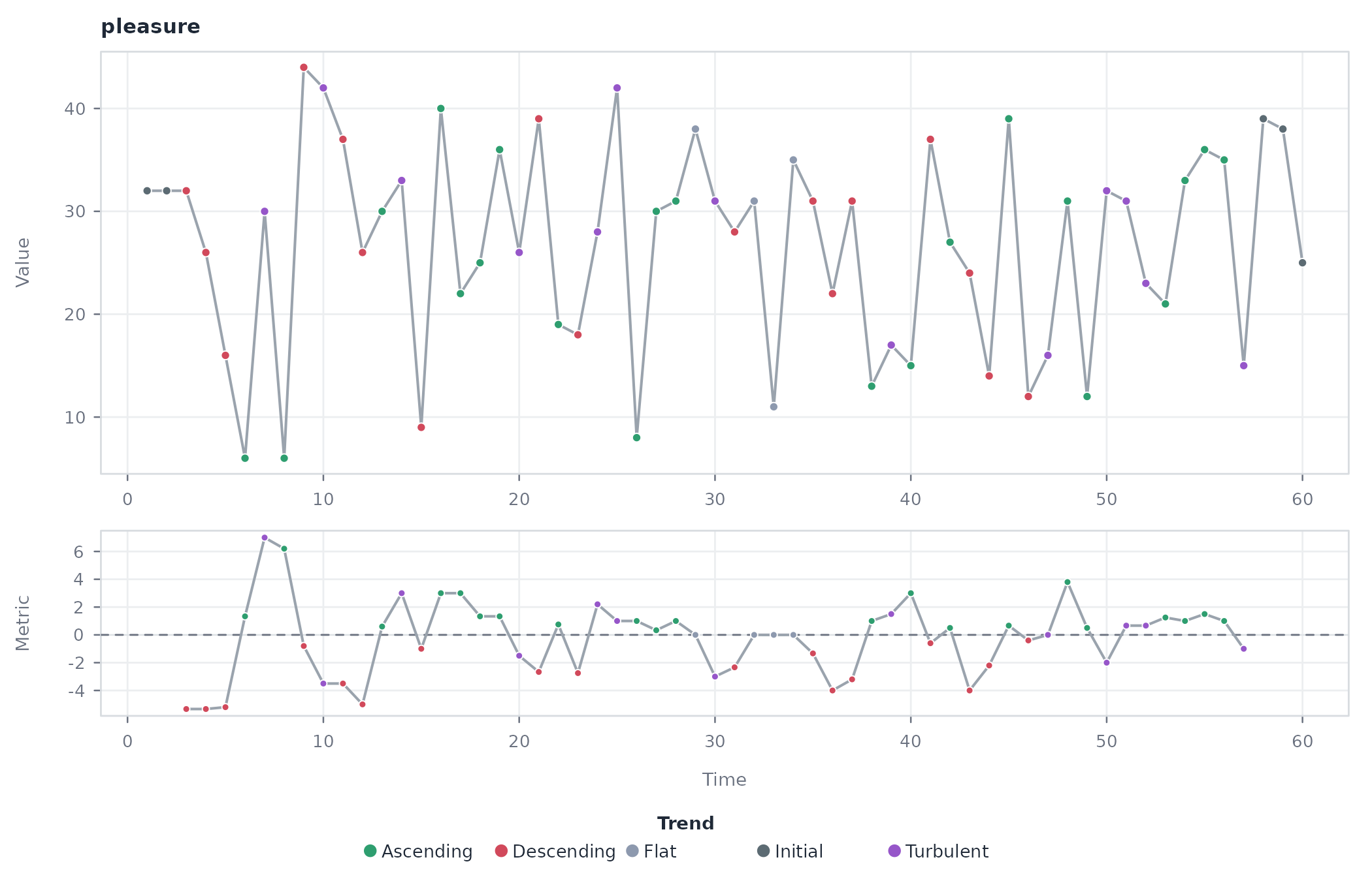

Two stacked panels: the pleasure series on top and its rolling slope metric below, with a shaded flat band marking near-zero slope.

The panel view places the rolling metric below the measurements, so the points at which the metric crosses the flat band can be checked against the assigned direction.

Visibility with `vg()`

vg() treats each observation as a node. Under natural visibility, two points are joined when the straight line between their values stays above every intervening point. Under horizontal visibility, they are joined only when every intervening value lies below both endpoints, a strictly stronger condition.

natural <- vg(
  data = pleasure,
  series = "pleasure"
)

summary(natural)
#>       method unit nodes dyads edges    density minimum_weight maximum_weight
#> 1 visibility time    60   143   143 0.08079096              1              1
#>   directed
#> 1    FALSE

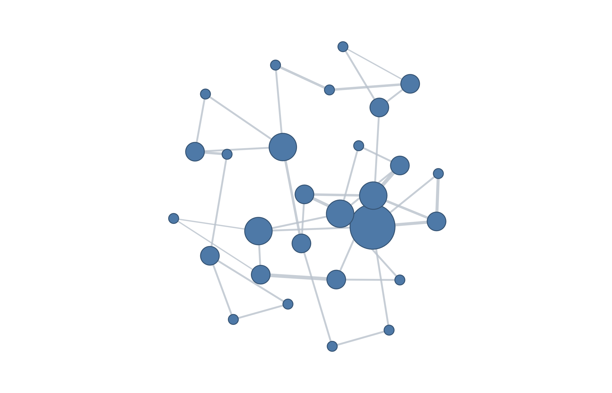
The natural visibility graph has 60 nodes and 143 edges. At this length the edges remain distinguishable, so it can be drawn directly. Node size encodes degree, and the peaks accumulate the most connections because they stay visible over the smaller values around them.

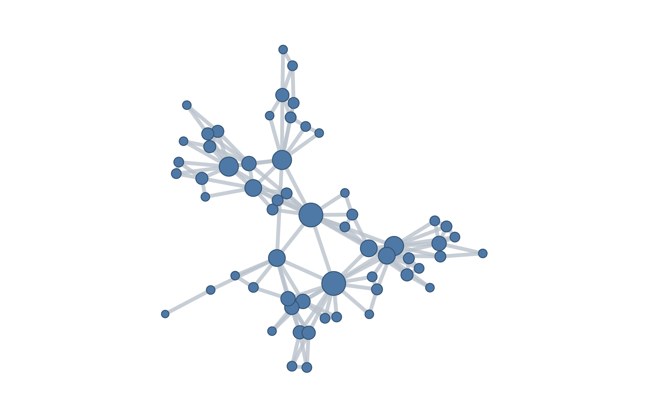
plot(natural, layout = "fr", node_size_range = c(1.4, 4.5))

Natural visibility graph of sixty pleasure observations, drawn with a Fruchterman-Reingold layout and nodes sized by degree; the high-degree hubs correspond to peaks that see far along the series, spread apart so individual nodes stay distinguishable.

The horizontal rule keeps the same 60 nodes but fewer edges.

horizontal <- vg(
  data = pleasure,
  type = "horizontal",
  series = "pleasure"
)

summary(horizontal)
#>       method unit nodes dyads edges    density minimum_weight maximum_weight
#> 1 visibility time    60   107   107 0.06045198              1              1
#>   directed
#> 1    FALSE

It retains 107 of the 143 connections, removing the 36 that a natural line of sight can clear but a horizontal one cannot. The result keeps the temporal chain of consecutive observations while dropping the longer sightlines that only the natural view permits. In both graphs the edge weights are binary, since visibility either holds or it does not.

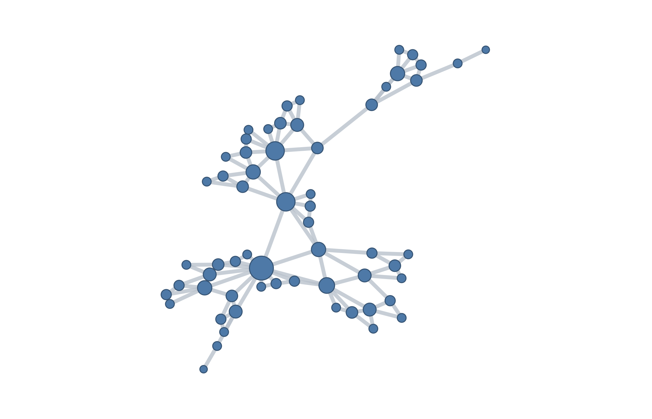
plot(horizontal, layout = "fr", node_size_range = c(1.4, 4.5))

Horizontal visibility graph of the same sixty observations, drawn with the same Fruchterman-Reingold layout and degree-scaled nodes; it is sparser than the natural graph, with the temporal chain visible alongside a smaller number of longer edges.

Every network also retains the series it was built from, which the source-series view recovers.

plot(horizontal, type = "series")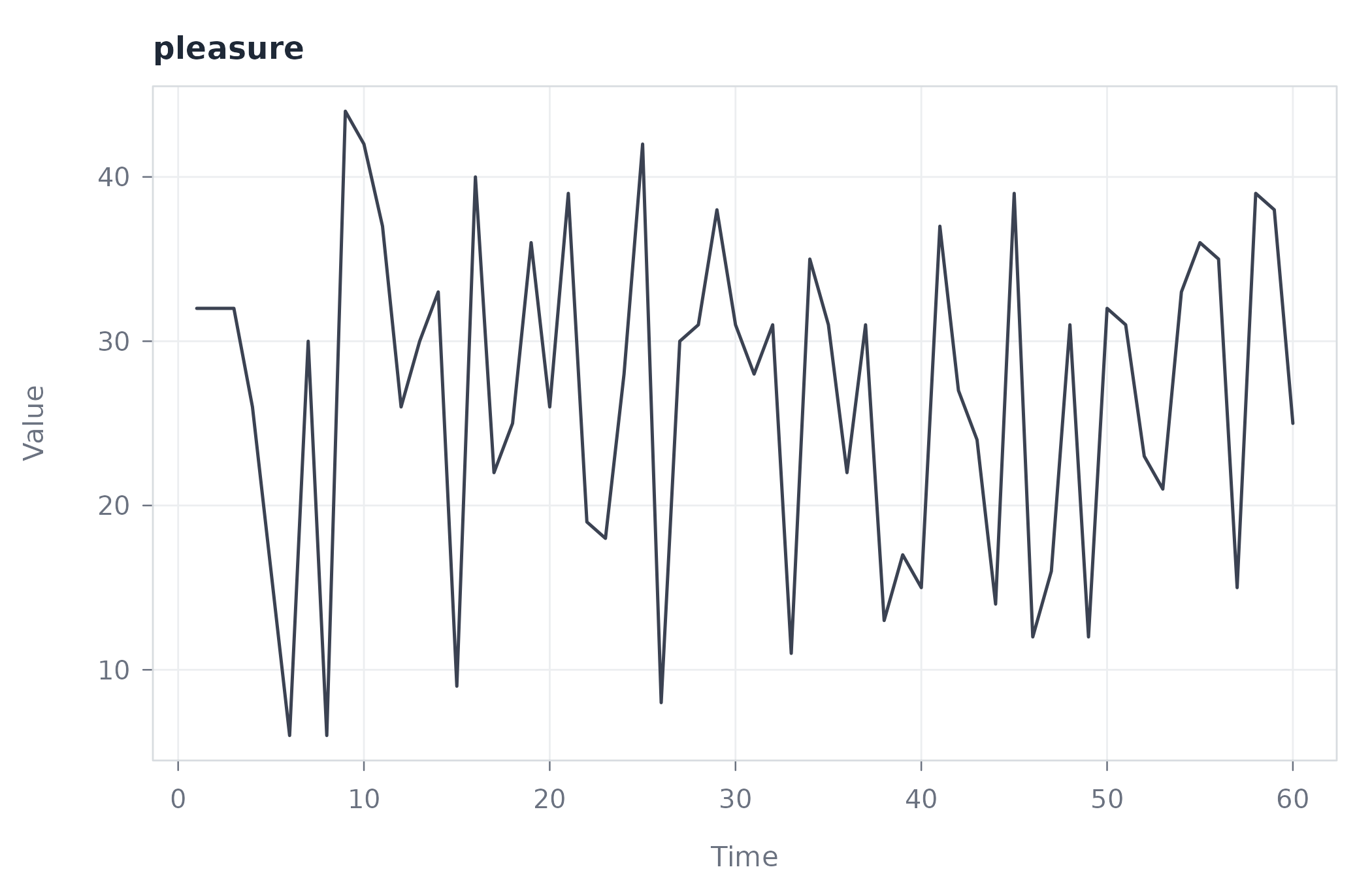

The sixty pleasure observations behind the visibility graph, plotted as a line over observation order.

This view makes the short-run fluctuation that the visibility rule reads directly apparent.

Window similarity with `tsn()`

tsn() is the general distance-network constructor. With method = "distance" a single measured series defaults to sliding-window nodes. The window width defaults to one tenth of the series length, which is 6 here, and a step of 2 yields 28 overlapping windows.

windows <- tsn(
  data = pleasure,
  method = "distance",
  series = "pleasure",
  step = 2
)

summary(windows)
#>     method   unit nodes dyads edges density minimum_weight maximum_weight
#> 1 distance window    28   378   378       1     0.01682183      0.1118912
#>   directed
#> 1    FALSE

The default full connection rule evaluates and keeps all 378 window pairs. Each edge weight is 1 / (1 + distance), so larger weights mark more similar windows.

sparse <- tsn(
  data = pleasure,
  method = "distance",
  series = "pleasure",
  step = 2,
  connect = "nearest",
  neighbors = 2
)

summary(sparse)
#>     method   unit nodes dyads edges   density minimum_weight maximum_weight
#> 1 distance window    28   378    40 0.1058201     0.03137678      0.1118912
#>   directed
#> 1    FALSE

Nearest-neighbour sparsification keeps 40 edges and lowers the density from 1 to 0.106, retaining the strongest local similarities instead of drawing every pair.

plot(sparse)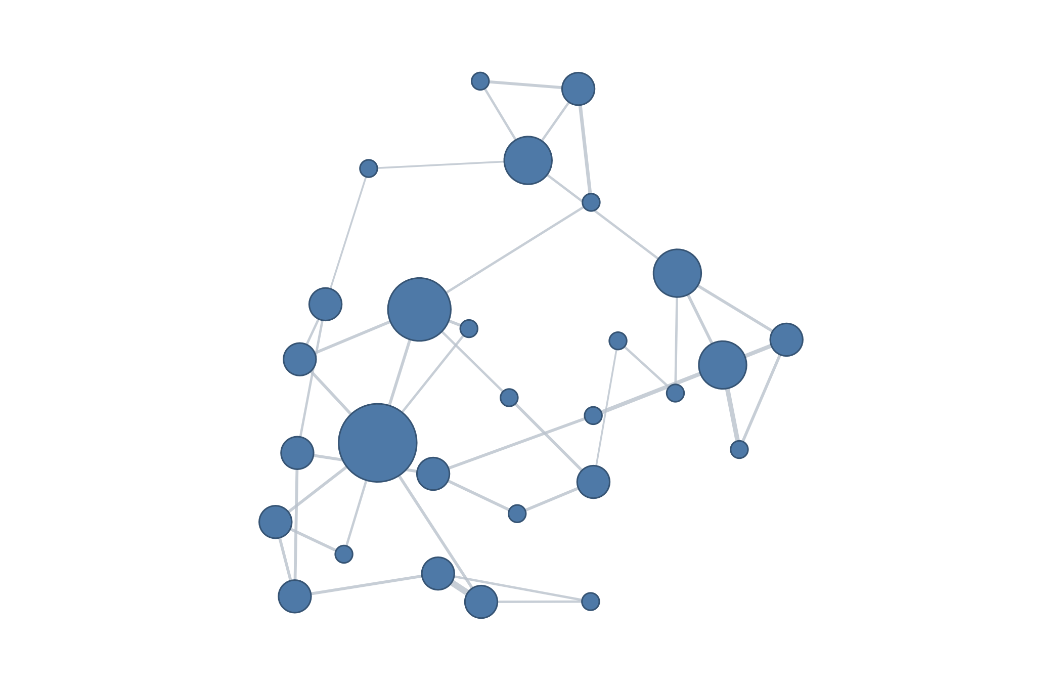

Nearest-neighbour distance network over twenty-eight sliding windows of the pleasure series, with edges joining the most similar windows.

No retained edge joins immediately adjacent windows. The closest retained pairs are two windows apart and the most distant are twenty-one windows apart, which shows that overlap in time does not by itself determine similarity in value: windows far apart in the sequence can still be each other’s nearest neighbours.

The distance measure is itself a modelling choice. Dynamic time warping aligns two windows by their shape, tolerating the shift or stretch in time that Euclidean distance penalizes. Repeating the sparsification under distance = "dtw" redraws the neighbour graph on the same 28 windows.

warped <- tsn(
  data = pleasure,
  method = "distance",
  series = "pleasure",
  step = 2,
  distance = "dtw",
  connect = "nearest",
  neighbors = 2
)

summary(warped)
#>     method   unit nodes dyads edges   density minimum_weight maximum_weight
#> 1 distance window    28   378    39 0.1031746     0.01851852     0.05555556
#>   directed
#> 1    FALSE

The warped network keeps 39 edges, almost as many as the Euclidean version’s 40, yet it connects largely different pairs of windows. Whether two windows count as similar therefore depends as much on the chosen distance as on the series itself.

plot(warped)

Nearest-neighbour distance network over the same twenty-eight windows using dynamic time warping, connecting a different set of window pairs than the Euclidean network.

Mohammed Saqr

Sonsoles López-Pernas

Manuel J. Gómez

Introduction

Data

Transition Network Analysis

Transition probabilities with `ts_tna()`

Transition frequencies with `ts_ftna()`

State co-occurrence with `ts_cna()`

Attention-weighted transitions with `ts_atna()`

Indexing the model with `series_networks()`

Local direction with `trend()`

Visibility with `vg()`

Window similarity with `tsn()`

Constructing Time Series Networks

Mohammed Saqr

Sonsoles López-Pernas

Manuel J. Gómez

Introduction

Data

Transition Network Analysis

Transition probabilities with ts_tna()

Transition frequencies with ts_ftna()

State co-occurrence with ts_cna()

Attention-weighted transitions with ts_atna()

Indexing the model with series_networks()

Local direction with trend()

Visibility with vg()

Window similarity with tsn()

Transition probabilities with `ts_tna()`

Transition frequencies with `ts_ftna()`

State co-occurrence with `ts_cna()`

Attention-weighted transitions with `ts_atna()`

Indexing the model with `series_networks()`

Local direction with `trend()`

Visibility with `vg()`

Window similarity with `tsn()`