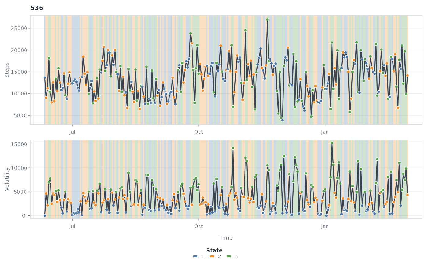
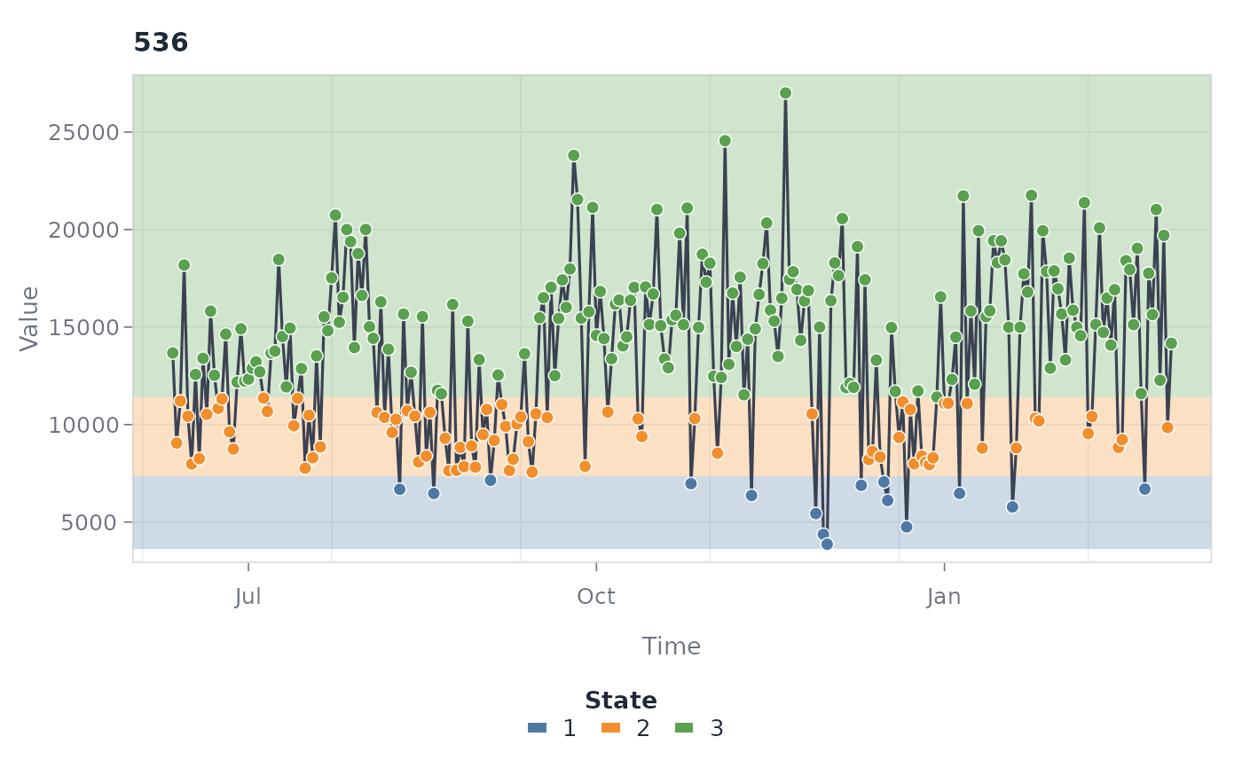
Plot a state discretization — plot.tsn

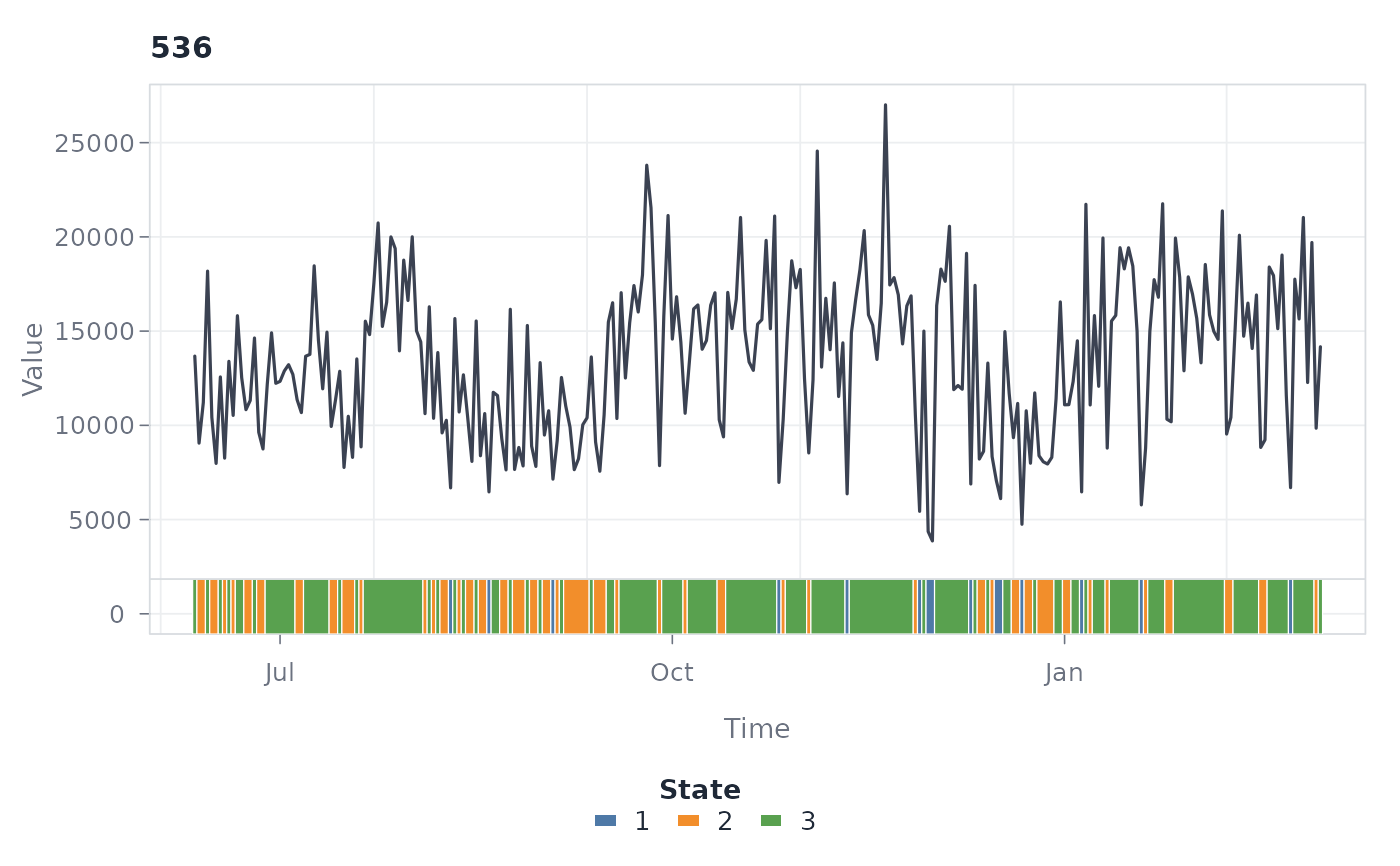
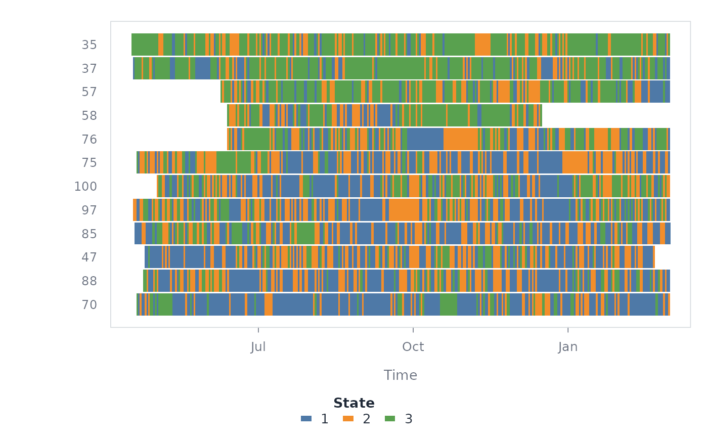
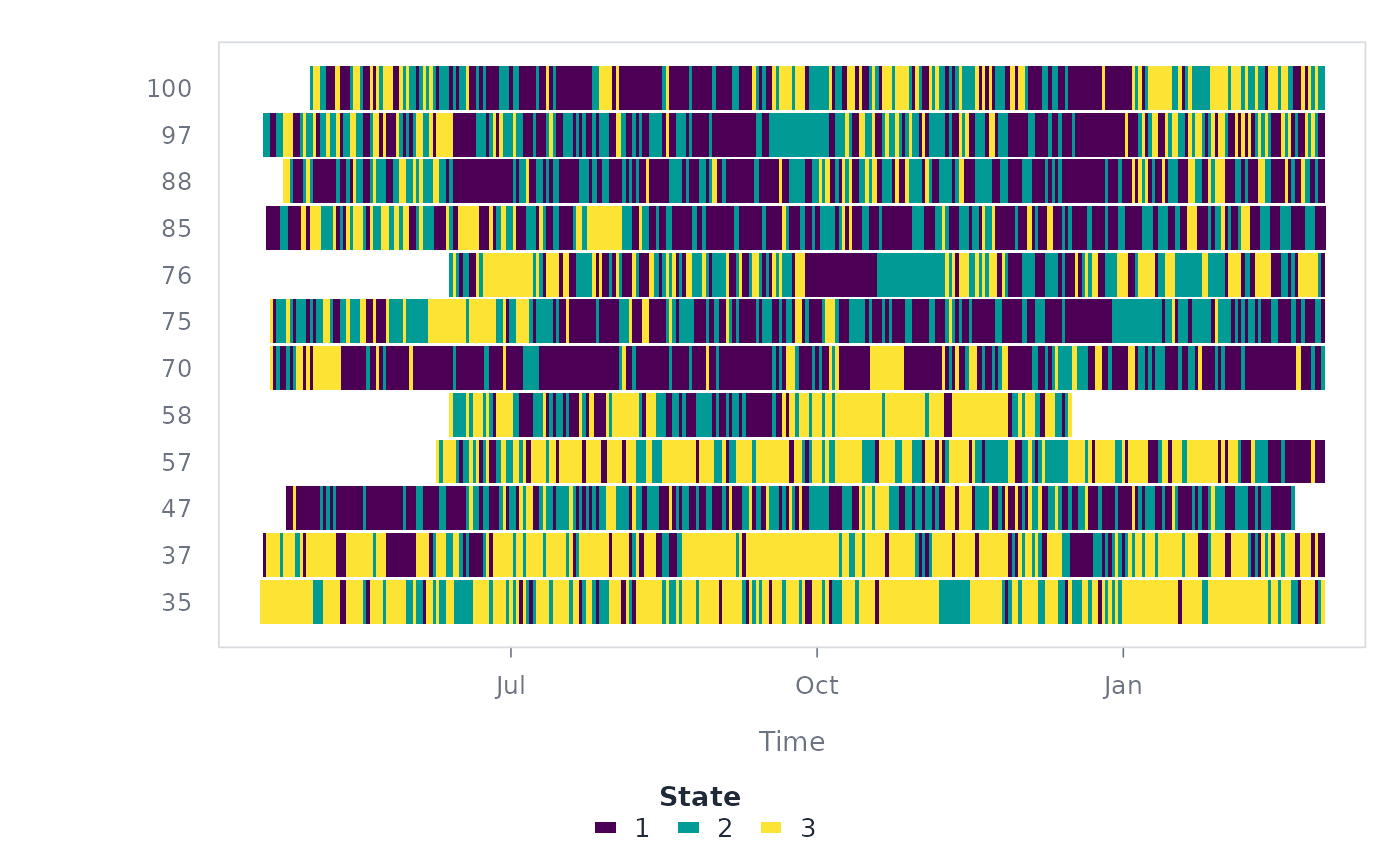
Four views of a discretized series, selected with type. "overlay" (default) draws each series with translucent state shading behind it; "ribbon" keeps the series clean and runs a state-classification strip underneath it instead; "heatmap" draws one row per series with one coloured tile per observation, which scales to many series where the faceted views do not; "stack" places an aligned companion series above the discretized series.

Usage

# S3 method for class 'tsn_states'
plot(
  x,
  type = c("overlay", "ribbon", "heatmap", "stack"),
  series = NULL,
  overlay = c("horizontal", "vertical", "none"),
  lines = "none",
  min_run = 1L,
  points = TRUE,
  max_series = NULL,
  columns = NULL,
  palette = NULL,
  alpha = NULL,
  line_color = "#3B4252",
  line_width = 1.6,
  point_size = 1,
  strip_height = 0.1,
  sort = "none",
  border = FALSE,
  with = NULL,
  with_label = "Series",
  shade = TRUE,
  color_line = FALSE,
  ribbons = NULL,
  ribbon_label = "States",
  legend = TRUE,
  xlab = "Time",
  ylab = "Value",
  cex = 1,
  grid = TRUE,
  background = "#FFFFFF",
  ...
)

Arguments

x: A tsn_states result.
type: The view: "overlay", "ribbon", "heatmap", or "stack". The stack view draws a companion series (with) above the discretized series with BOTH panels vertically shaded by the discretized states — e.g. the original time series read against the states of its rolling complexity.
series: Optional character vector of series IDs to display.
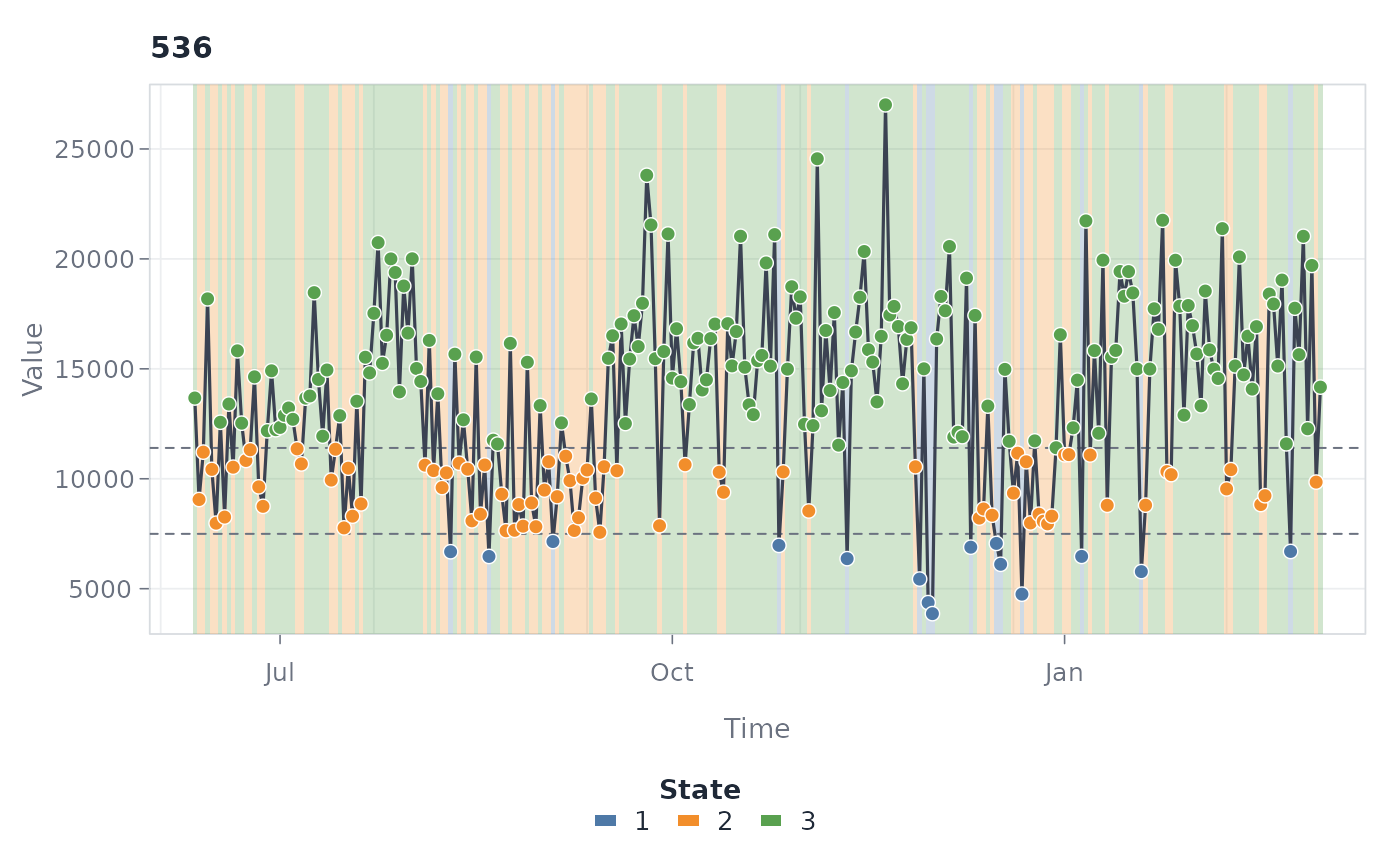
overlay: Colour shading for the overlay view: "horizontal" (default; value bands), "vertical" (time runs), or "none".
lines: Dashed guide lines complementing the shading: "horizontal" draws grey lines at the state boundaries (the discretization breaks when available, empirical boundaries otherwise). Transformed and magnitude-space breaks are converted back to the raw signed value axis; adaptive local boundaries are omitted. "vertical" draws a line at each state transition (filtered by min_run) in the colour of the state that starts there — a green dashed line means the green state begins at that point and runs until the next line; "both", or "none" (default). Combine one shading direction with dashed lines in the other, e.g. overlay = "horizontal", lines = "vertical".
min_run: For lines = "vertical": only transitions into a state persisting at least min_run observations get a line.
points: Whether to draw observations over each line.
max_series: Maximum number of series to draw (25 for the heatmap, 10 otherwise).
columns: Number of panel columns.
palette: State colours: NULL for the default palette, a preset name ("default", "okabe", "viridis", "cool", "warm", "pastel", "dark"), a named colour vector keyed by state, or a plain colour vector.
alpha: Shading opacity for the overlay view.
line_color: Series line colour.
line_width: Series line width.
point_size: Observation point size.
strip_height: Height of the ribbon strip as a fraction of the panel.
sort: Heatmap row order: "none", "mean" (by series mean value), or "state" (group rows by modal state).
border: Whether heatmap tiles carry a thin separator border.
with: For type = "stack": a finite numeric vector aligned with the rows of x giving the companion series (e.g. the original values when x discretizes a derived series).
with_label: Y-axis title of the companion panel.
shade: For type = "stack": whether to draw the vertical state shading on both panels.
color_line: For type = "stack": colour each line segment by the state at its left endpoint instead of drawing a neutral line.
ribbons: For type = "ribbon": an optional NAMED list of additional classifications to stack below the series — each element a tsn_states, a trend() result, or a character/factor vector aligned with the selected series. The object's own states form the first strip (labelled ribbon_label); one series at a time. This is the resilience-style multi-ribbon view: the series read against several classifications at once, each strip labelled on the axis with its own legend row.
ribbon_label: Strip label for the object's own states in the multi-ribbon view.
legend: Whether to draw the legend row.
xlab, ylab: Axis titles.
cex: Global text size multiplier.
grid: Whether to draw the background grid.
background: Panel background colour.
...: Reserved for future options.

Value

x, invisibly.

Examples

data(steps)
complete <- subset(steps, !is.na(steps))
states <- discretize(
  complete,
  value = "steps", id = "id", time = "day",
  method = "quantile", n_states = 3
)
plot(states, series = "536")

plot(states, series = "536", overlay = "vertical", lines = "horizontal")

plot(states, "ribbon", series = "536", points = FALSE)

plot(states, "heatmap", max_series = 12, sort = "mean")

plot(states, "heatmap", palette = "viridis", max_series = 12)


# Stack: original series read against the states of its rolling volatility.
one <- subset(complete, id == 536)
volatility <- abs(c(0, diff(one$steps)))
vol_states <- discretize(
  data.frame(id = one$id, day = one$day, vol = volatility),
  value = "vol", id = "id", time = "day",
  method = "quantile", n_states = 3
)
plot(vol_states, "stack", with = one$steps, with_label = "Steps",
     ylab = "Volatility")