Plot a TSN Result

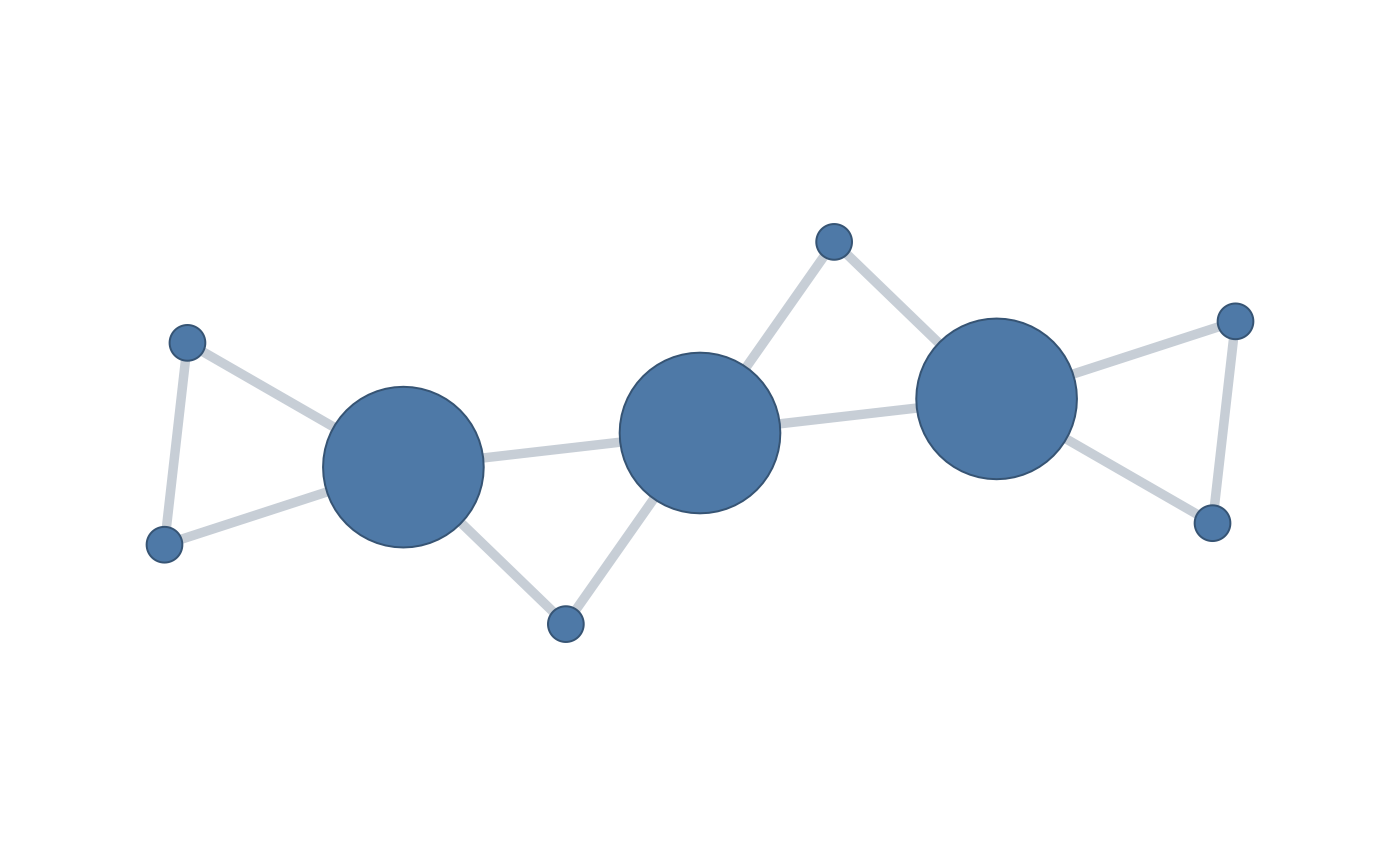
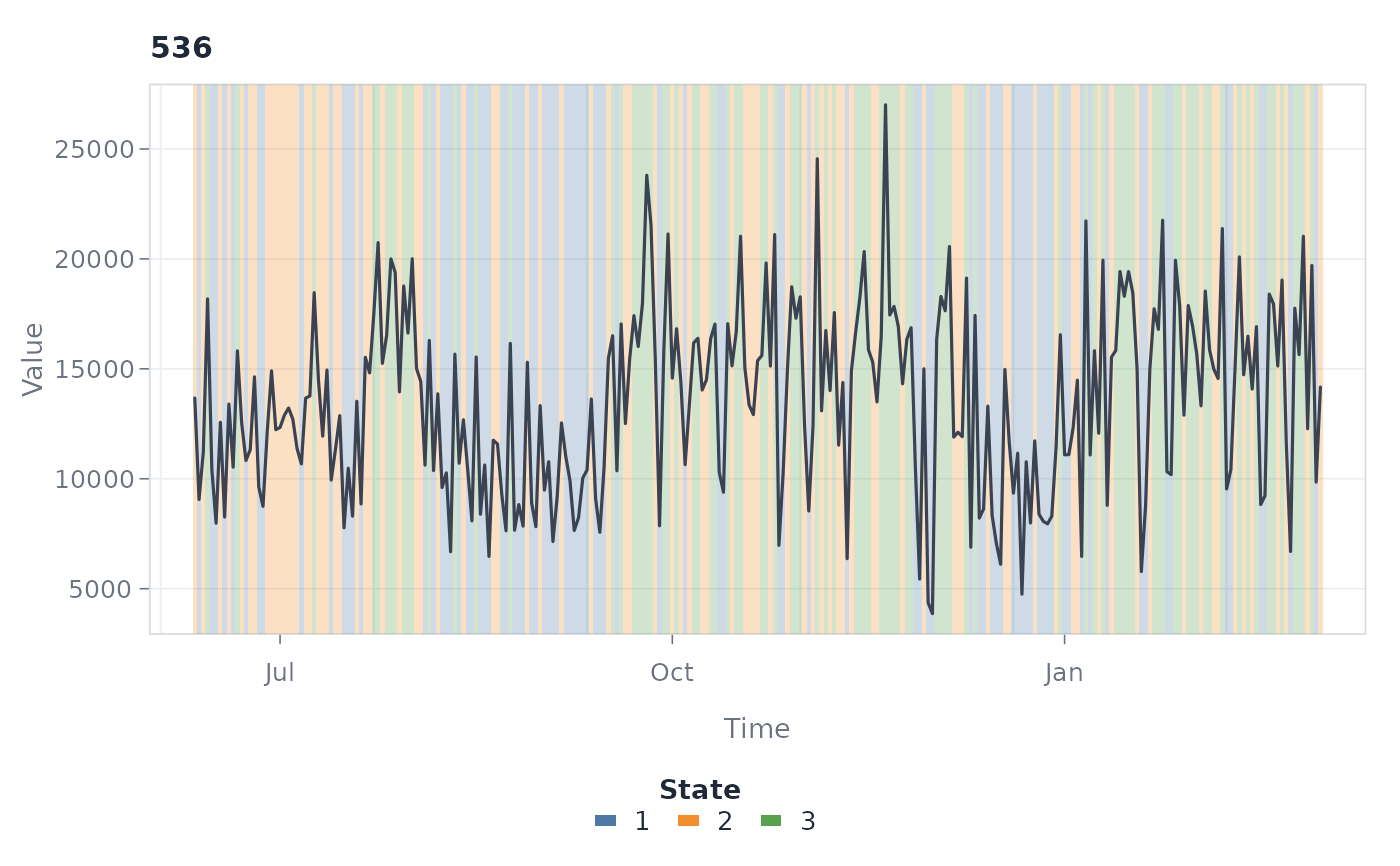
By default, plot() renders the constructed network through cograph::splot(). The diagnostic source-series view (with optional state shading) remains available via type = "series" and does not require cograph.

Usage

# S3 method for class 'tsn'
plot(x, type = c("network", "series"), ...)

Arguments

x

A tsn result.

type

What to draw: "network" (default) or "series".

...

Arguments forwarded to the network or series renderer. See details.

Value

x, invisibly.

Details

Network rendering belongs exclusively to cograph. tsn supplies restrained defaults that keep edges visible and avoid meaningless per-node rainbow fills; named arguments in ... override any of them. tsn results already implement the cograph_network contract. Source-series views remain tsn-specific because they visualize the original observations rather than a generic network.

For type = "network", use cograph arguments such as layout, labels, scale_nodes_by, node_size_range, and edge_label_style. For type = "series", ... accepts series, overlay, points, trend, columns, max_series, scales, and palette.

Examples

network <- tsn(c(3, 1, 4, 2, 5, 3, 6, 2, 7), "hvg")
if (requireNamespace("cograph", quietly = TRUE)) {
  plot(network)
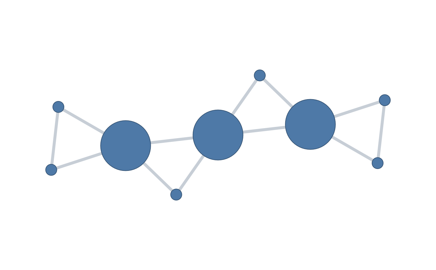
  plot(network, layout = "spring")
}



data(steps)
states <- tsn(
  steps,
  value = "steps",
  id = "id",
  time = "day",
  series = 536,
  unit = "state",
  discretization = "quantile"
)
plot(states, "series", overlay = "vertical")