4. Advanced analysis: smoothing, tuning, comparison, and mining
Source:vignettes/advanced-analysis.Rmd
advanced-analysis.RmdThis vignette covers the parts of transitiontrees beyond
the basic fit-prune-predict loop: choosing a smoother and a pruning
rule, picking hyperparameters by cross-validation, quantifying pathway
reliability, comparing cohorts with a permutation test, introspecting
the fitted tree, and mining it for contexts and sequences of
interest.
Setup
We work throughout from one fit on the bundled
trajectories data and its pruned form – the same starting
point as Getting started.
library(transitiontrees)
data(trajectories)
set.seed(1)

tree   <- context_tree(trajectories, max_depth = 4L, min_count = 5L)
pruned <- prune_tree(tree, criterion = "G2", alpha = 0.05)
1. Smoothing schemes
Smoothing decides what probability an unseen next state
receives. Five schemes are implemented (floor,
laplace, kneser_ney, witten_bell,
jelinek_mercer). compare_smoothing() refits
under each and reports in-sample perplexity in one call.
compare_smoothing(trajectories, max_depth = 4L, min_count = 5L)
#>        smoothing n_nodes perplexity
#> 1          floor      82   2.157411
#> 2        laplace      82   2.181832
#> 3     kneser_ney      82   2.167730
#> 4    witten_bell      82   2.161948
#> 5 jelinek_mercer      82   2.200473
Two things to read. First, n_nodes is identical across
schemes – smoothing changes probabilities, never which
contexts exist; topology is set by min_count, not the
smoother. Second, do not pick a smoother on in-sample
perplexity (it rewards memorisation); the cross-validation in section 3
is the verdict that counts.
Handed a fitted tree, compare_smoothing()
re-smooths it under every scheme (via smooth_tree(),
without re-counting) instead of refitting – a smoothing sweep on the
already-pruned model in one call:
compare_smoothing(pruned)
#>        smoothing n_nodes perplexity
#> 1          floor      25   2.239207
#> 2        laplace      25   2.243759
#> 3     kneser_ney      25   2.241328
#> 4    witten_bell      25   2.240596
#> 5 jelinek_mercer      25   2.296256
2. Pruning criteria
prune_tree() supports four criteria.
compare_pruning() applies each – holding
alpha/threshold fixed – and reports how hard
each one trims.
compare_pruning(tree)
#>   criterion n_nodes reduction_pct
#> 1        G2      25          69.5
#> 2        KL      78           4.9
#> 3       AIC      42          48.8
#> 4       BIC      36          56.1
G2 (the likelihood-ratio test) and AIC ask
“is the extra depth justified given its sample size?”; BIC
punishes parameters harder (its penalty scales with log n);
KL at a lenient absolute threshold keeps
almost everything. Use G2 (or AIC) unless you
have a specific reason, and report the reduction – “most grown contexts
were unjustified” is itself a finding.
3. Cross-validated tuning
tune_tree() runs k-fold CV at the sequence
level over a grid of
(max_depth, min_count, smoothing, prune) and returns a
ranked data.frame with the winner on attr(., "best").
tg <- tune_tree(trajectories, max_depth = 1L:4L, folds = 5L, seed = 42L)
head(tg, 6)
#> <transitiontrees_tune>  6 configurations
#>  max_depth nmin                           smoothing prune    logLik n_scored
#>          4   10 floor(ymin=0.001, rule=interpolate) FALSE -1568.594     1870
#>          3   10 floor(ymin=0.001, rule=interpolate) FALSE -1578.793     1870
#>          4   10 floor(ymin=0.001, rule=interpolate)  TRUE -1580.100     1870
#>          3   10 floor(ymin=0.001, rule=interpolate)  TRUE -1582.190     1870
#>          2    3 floor(ymin=0.001, rule=interpolate) FALSE -1583.660     1870
#>          2    5 floor(ymin=0.001, rule=interpolate) FALSE -1583.660     1870
#>  perplexity n_nodes_avg folds_failed
#>    2.313636        59.8            0
#>    2.326290        31.2            0
#>    2.327916        23.4            0
#>    2.330519        15.4            0
#>    2.332352        13.0            0
#>    2.332352        13.0            0
#>
#> best (min perplexity):
#>  max_depth nmin                           smoothing prune    logLik n_scored
#>          4   10 floor(ymin=0.001, rule=interpolate) FALSE -1568.594     1870
#>  perplexity n_nodes_avg folds_failed
#>    2.313636        59.8            0
attr(tg, "best")
#>   max_depth nmin                           smoothing prune    logLik n_scored
#> 1         4   10 floor(ymin=0.001, rule=interpolate) FALSE -1568.594     1870
#>   perplexity n_nodes_avg folds_failed
#> 1 2.313636 59.8 0(min_count and prune are swept by their
defaults; add smoothing = or a wider
min_count = to grow the grid.)
plot(tg)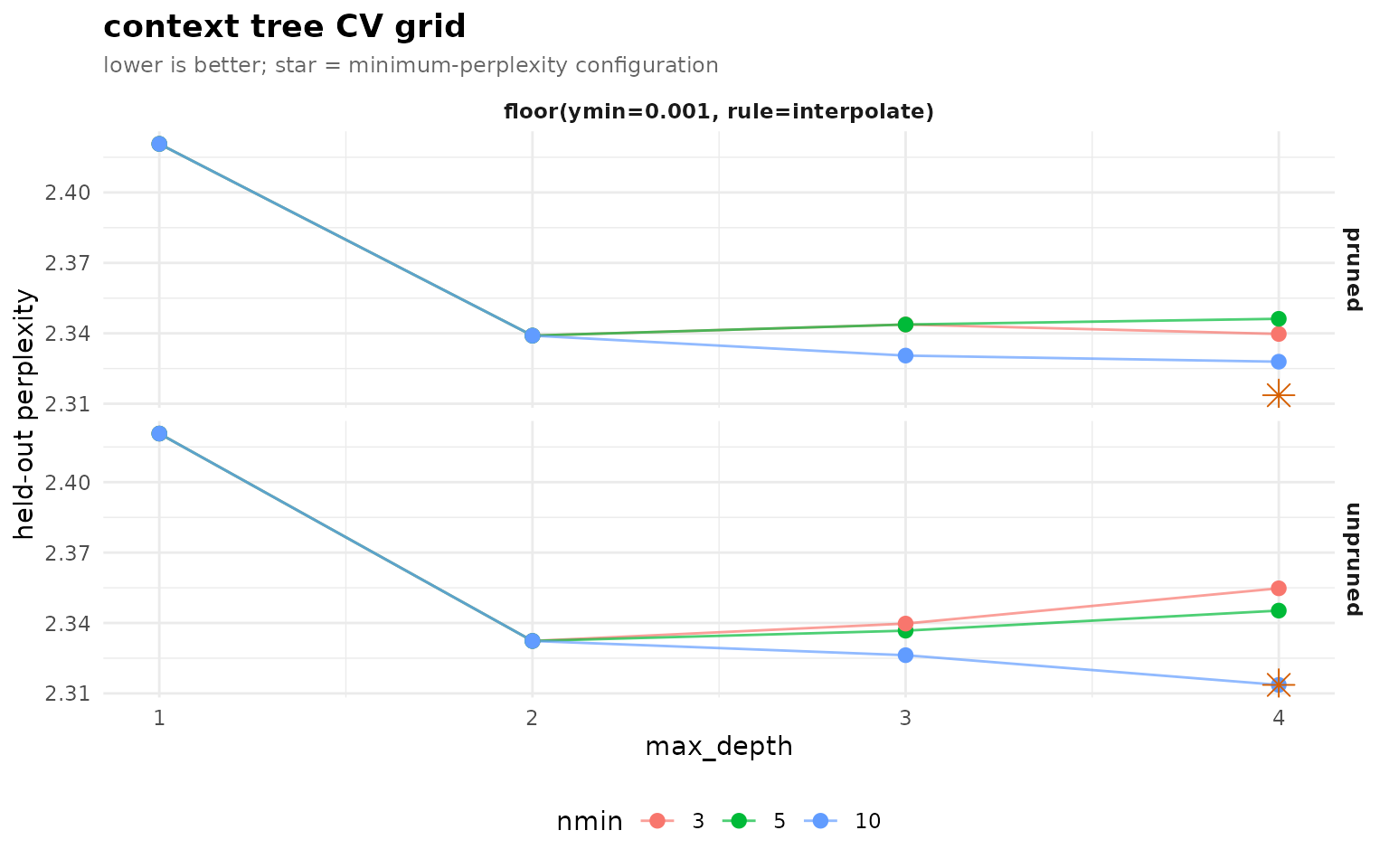
The shape of the curve is as informative as the winning point: if
perplexity keeps falling with max_depth the process has
long memory; if it flattens early (as engagement data tends to) the
useful memory is short and deeper trees just overfit. Refit at the
chosen configuration on the full data for downstream use.
4. Bootstrap pathway reliability
bootstrap_pathways() resamples whole sequences and
reports, per pathway, stability_rate (the count reproduces)
and informative_rate (the G-squared against the parent
reproducibly clears the chi-square bar). Keeping the raw resamples lets
you also see the full distribution of any statistic.
boot <- bootstrap_pathways(pruned, iter = 200L, stat = "count",
                          seed = 1L, keep_resamples = TRUE)
boot
#> <transitiontrees_bootstrap>  200 resamples
#>   stability  : count in [0.50, 1.50] x observed, p < 0.05
#>   informative: G^2 > qchisq(0.95, df=k-1) = 5.99, threshold 0.80
#>   pathways   : 25 total, 22 stable, 16 informative, 15 both
#>
#> top pathways (stable + informative first):
#>                                pathway depth count p_stability stability_rate
#>                                Average     1   751       0.005              1
#>                                 Active     1   658       0.005              1
#>                       Active -> Active     2   433       0.005              1
#>                             Disengaged     1   325       0.005              1
#>                      Active -> Average     2   160       0.005              1
#>                      Average -> Active     2   144       0.005              1
#>                  Disengaged -> Average     2   122       0.005              1
#>           Active -> Average -> Average     3    80       0.005              1
#>            Average -> Active -> Active     3    70       0.005              1
#>  Average -> Active -> Active -> Active     4    37       0.005              1
#>  stable informative_rate informative mean_G2 ci_G2_lo ci_G2_hi
#>    TRUE            1.000        TRUE 118.478   75.640  167.234
#>    TRUE            1.000        TRUE 320.221  252.539  400.370
#>    TRUE            0.990        TRUE  17.883    7.760   29.091
#>    TRUE            1.000        TRUE 180.794  112.545  264.322
#>    TRUE            1.000        TRUE  28.771   13.505   44.901
#>    TRUE            1.000        TRUE  30.211   11.246   51.521
#>    TRUE            1.000        TRUE  32.634   14.488   53.156
#>    TRUE            0.875        TRUE  13.152    2.924   26.802
#>    TRUE            0.990        TRUE  24.345    9.173   44.483
#>    TRUE            0.860        TRUE  13.638    2.414   32.937
#> # ... 15 more pathways (use summary(x) for full table)
summary() returns the tidy per-pathway table, sorted so
the trustworthy (stable and informative) pathways come first.
Each tracked statistic (count,
next_probability, divergence, G2)
carries a symmetric mean / sd / ci_lo / ci_hi quartet, so
you can report a bootstrap CI for any pathway statistic rather than a
bare point estimate:
head(summary(boot))
#>             pathway depth count likely_next next_probability divergence
#> 1           Average     1   751     Average        0.6098535 0.11356246
#> 2            Active     1   658      Active        0.6975684 0.34948716
#> 3  Active -> Active     2   433      Active        0.7852194 0.02860157
#> 4        Disengaged     1   325  Disengaged        0.4830769 0.40306556
#> 5 Active -> Average     2   160     Average        0.5187500 0.12282588
#> 6 Average -> Active     2   144      Active        0.5000000 0.14727560
#>   changes_prediction        G2 p_stability stability_rate stable
#> 1              FALSE 118.23068 0.004975124              1   TRUE
#> 2               TRUE 318.79579 0.004975124              1   TRUE
#> 3              FALSE  17.16853 0.004975124              1   TRUE
#> 4               TRUE 181.59944 0.004975124              1   TRUE
#> 5              FALSE  27.24365 0.004975124              1   TRUE
#> 6              FALSE  29.40010 0.004975124              1   TRUE
#>   informative_rate informative flip_consistency mean_count sd_count ci_count_lo
#> 1             1.00        TRUE            0.885    752.070 49.62366      652.95
#> 2             1.00        TRUE            0.885    657.700 55.88071      550.90
#> 3             0.99        TRUE            1.000    433.105 49.77925      347.75
#> 4             1.00        TRUE            0.785    326.365 33.36492      265.00
#> 5             1.00        TRUE            0.950    159.290 13.32115      136.00
#> 6             1.00        TRUE            0.620    143.935 13.10494      121.95
#>   ci_count_hi mean_next_probability sd_next_probability ci_next_probability_lo
#> 1     844.325             0.6074684          0.02383435              0.5602254
#> 2     769.175             0.6970828          0.02745211              0.6442147
#> 3     535.200             0.7840172          0.02690600              0.7281187
#> 4     396.050             0.4872506          0.03622112              0.4314732
#> 5     183.050             0.5208427          0.03928445              0.4550557
#> 6     168.025             0.5250488          0.02598869              0.4843571
#>   ci_next_probability_hi mean_divergence sd_divergence ci_divergence_lo
#> 1              0.6549035      0.11439634    0.02594025       0.07183403
#> 2              0.7533809      0.35344122    0.05055127       0.26995876
#> 3              0.8310155      0.03012959    0.01054014       0.01320413
#> 4              0.5611873      0.39995240    0.08188558       0.26407728
#> 5              0.5894276      0.13121723    0.04498657       0.05884796
#> 6              0.5811224      0.15297707    0.05681028       0.05396748
#>   ci_divergence_hi   mean_G2     sd_G2  ci_G2_lo  ci_G2_hi
#> 1       0.16703707 118.47766 24.209041  75.64028 167.23404
#> 2       0.44497422 320.22058 39.049877 252.53941 400.37042
#> 3       0.05071584  17.88321  5.887328   7.75980  29.09055
#> 4       0.57174185 180.79424 40.744883 112.54453 264.32204
#> 5       0.21775813  28.77083  9.600579  13.50545  44.90087
#> 6       0.26903470  30.21052 10.582009  11.24551  51.52106
plot_pathway_resamples() draws the full resample
distribution per pathway. A tight unimodal peak means the estimate is
well-determined; a bimodal or heavy-tailed panel is the tell that the
pathway is carrier-driven – a few sequences account for it, and
dropping them in a resample collapses it.
plot_pathway_resamples(boot, stat = "divergence", top = 6L)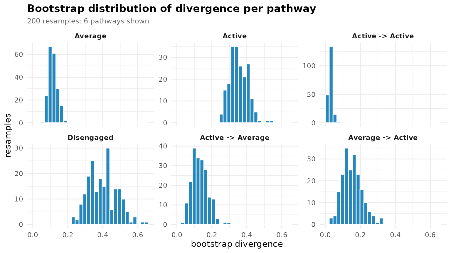
5. Comparing two cohorts
Name an external group column and
context_tree(group = ) fits one tree per group in a single
call, returning a transitiontrees_group that
prune_tree() and compare_trees() consume
directly – no manual splitting or label-building. We compare high- and
low-achieving students on the bundled group_regulation_long
log.
data(group_regulation_long)
grp <- prune_tree(context_tree(group_regulation_long,
                              actor = "Actor", time = "Time", action = "Action",
                              group = "Achiever", max_depth = 2L, min_count = 10L))
cmp <- compare_trees(grp, iter = 199L, seed = 1L)
cmp
#> <transitiontrees_comparison>  iter = 199
#>   observed distance : 0.0478
#>   null mean         : 0.00368
#>   p-value           : 0.005
#>
#> top divergent pathways:
#>                pathway count_a count_b divergence_ab divergence_ba
#>   cohesion -> cohesion      40       0         0.473         0.447
#>              synthesis     278     374         0.300         0.311
#>     emotion -> emotion      86       0         0.133         0.251
#>                discuss    2003    1948         0.178         0.204
#>               cohesion     938     757         0.120         0.115
#>  discuss -> coregulate       0     170         0.096         0.080
#>  divergence_sym
#>           0.460
#>           0.305
#>           0.192
#>           0.191
#>           0.117
#>           0.088
The printed comparison reports the observed distance
(pdist, a count-weighted symmetric-KL between the cohorts’
pathway distributions) and the p_value from permuting the
sequence-to-cohort labels. A significant result says the cohorts
generate genuinely different pathway dynamics, not a relabelling
artefact.
plot(cmp)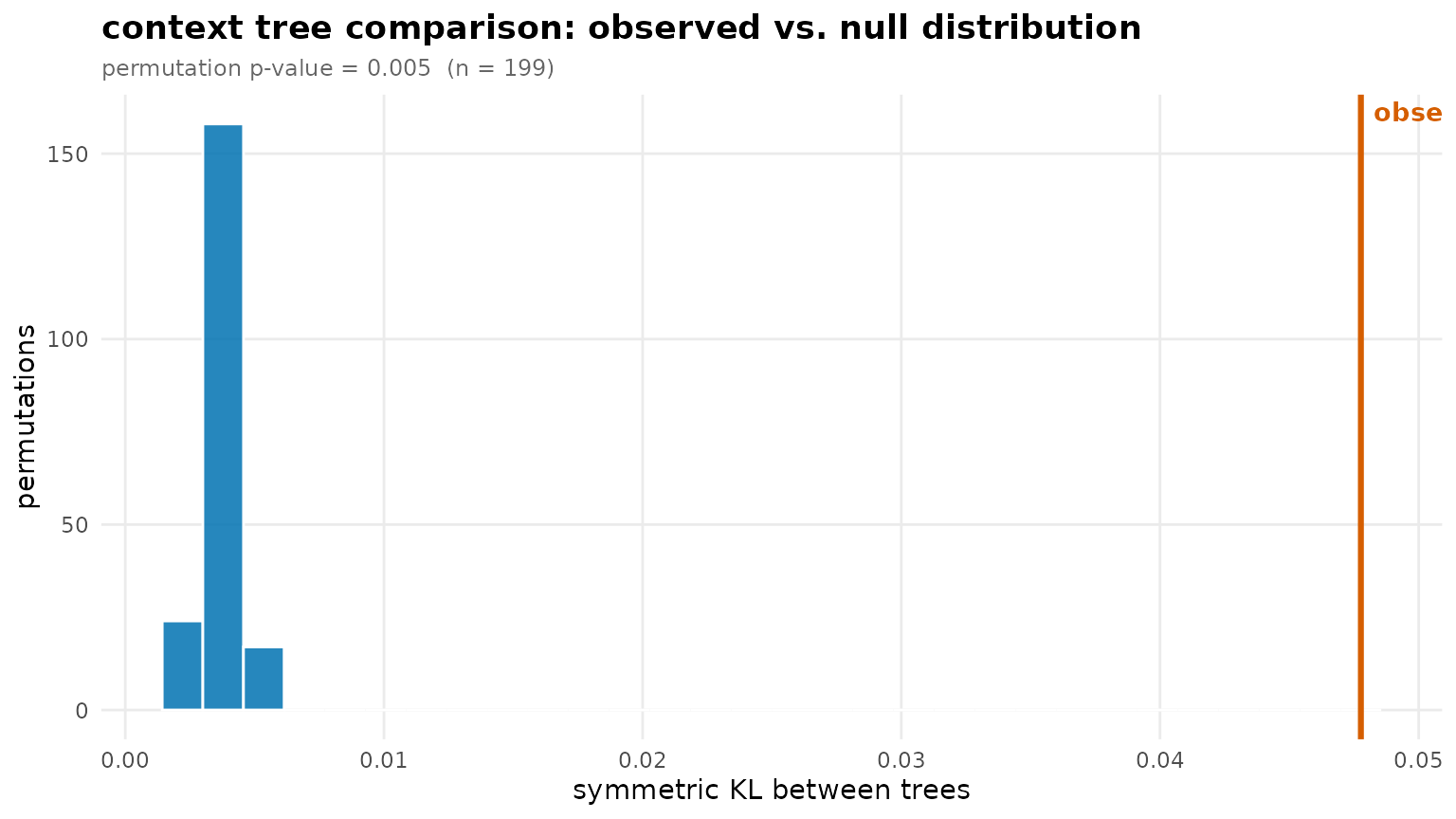
For the full per-axis decomposition (behavioural vs usage) and a tidy
pairwise distance_matrix, compare_groups()
consumes the same group =-fitted tree – see the
Complete analysis case vignette.
6. Tree introspection
Three accessors treat the tree as a queryable object.
query_pathway(pruned, c("Active", "Active"))               # full distribution
#>     Active    Average Disengaged
#> 0.78521940 0.19399538 0.02078522
query_pathway(pruned, "Disengaged", next_state = "Disengaged")  # one cell
#> [1] 0.4830769
pathway_exists(pruned, "Active -> Disengaged")             # membership (no backoff)
#> [1] TRUE
By default an unseen context backs off to its longest matching
suffix; pass exact = TRUE to demand the literal node
(returns NA if it is not one) – the tool for auditing
which contexts the tree actually holds.
query_pathway(pruned, c("Active", "Average", "Active"), exact = TRUE)
#>     Active    Average Disengaged
#>         NA         NA         NA
subtree() extracts the slice rooted at a context – the
same pathway API then runs on the slice:
sub <- subtree(pruned, "Active")   # its banner reads "subtree of: Active"
sub
#> <transitiontrees>  7 nodes, depth <= 4, 3 states  [pruned]
#>   alphabet : Active, Average, Disengaged
#>   fit on   : 136 sequences, 1870 observations
#>   smoothing: floor(ymin=0.001, rule=interpolate)   min_count = 5
#>   pruned by: G2   alpha = 0.05
#>   subtree of: Active
head(tree_pathways(sub), 4)
#>                      pathway depth count likely_next next_probability
#> 1                     Active     1   658      Active        0.6975684
#> 2           Active -> Active     2   433      Active        0.7852194
#> 3 Active -> Active -> Active     3   316      Active        0.8354430
#> 4          Average -> Active     2   144      Active        0.5000000
#>   divergence changes_prediction
#> 1         NA                 NA
#> 2 0.02860157              FALSE
#> 3 0.01149187              FALSE
#> 4 0.14727560              FALSE
7. Mining contexts and sequences
mine_contexts() scans the tree for contexts where a
chosen state is unusually likely (or unlikely):
mine_contexts(pruned, state = "Disengaged", min_prob = 0.5)
#>                                          pathway depth count      state
#> 1 Disengaged -> Average -> Average -> Disengaged     4    13 Disengaged
#> 2                       Disengaged -> Disengaged     2   139 Disengaged
#>        prob is_modal
#> 1 0.8461538     TRUE
#> 2 0.6762590     TRUE
mine_sequences() ranks supplied sequences by how well
the model predicts them – the surprising ones are atypical
trajectories worth a closer look:
mine_sequences(pruned, newdata = trajectories, which = "surprising", n = 5L)
#>   sequence_id n_scored   log_lik perplexity
#> 1          33        1 -1.664397   5.282486
#> 2          96        1 -1.664397   5.282486
#> 3          97        1 -1.664397   5.282486
#> 4         101        1 -1.664397   5.282486
#> 5         104        1 -1.664397   5.282486
8. Imputing gaps
impute_sequences() fills internal missing
states from the fitted tree – modal takes the most likely
state at each gap, prob samples from the predicted
distribution:
gappy <- list(c("Active", "Active", NA, "Disengaged"),
              c("Average", NA, "Average"))
impute_sequences(pruned, gappy, method = "modal")
#> [[1]]
#> [1] "Active"     "Active"     "Active"     "Disengaged"
#>
#> [[2]]
#> [1] "Average" "Average" "Average"
9. Generating sequences
Every fitted tree is also a generative model.
generate_sequences() samples by walking the conditional
distributions; simulate() is the R-standard generic
wrapping it with nsim and a seed.
generate_sequences(pruned, n = 4L, length = 10L)
#>      [,1]         [,2]         [,3]         [,4]         [,5]
#> [1,] "Average"    "Active"     "Active"     "Active"     "Active"
#> [2,] "Active"     "Active"     "Active"     "Active"     "Active"
#> [3,] "Disengaged" "Disengaged" "Disengaged" "Disengaged" "Disengaged"
#> [4,] "Active"     "Disengaged" "Average"    "Average"    "Average"
#>      [,6]         [,7]         [,8]         [,9]         [,10]
#> [1,] "Active"     "Active"     "Average"    "Disengaged" "Active"
#> [2,] "Average"    "Average"    "Average"    "Average"    "Average"
#> [3,] "Disengaged" "Disengaged" "Disengaged" "Disengaged" "Disengaged"
#> [4,] "Average"    "Active"     "Average"    "Active"     "Active"
simulate(pruned, nsim = 4L, seed = 42L, length = 10L)
#>      [,1]         [,2]         [,3]         [,4]         [,5]
#> [1,] "Disengaged" "Average"    "Disengaged" "Active"     "Disengaged"
#> [2,] "Disengaged" "Average"    "Disengaged" "Average"    "Average"
#> [3,] "Average"    "Active"     "Active"     "Active"     "Active"
#> [4,] "Disengaged" "Disengaged" "Average"    "Disengaged" "Disengaged"
#>      [,6]         [,7]      [,8]         [,9]         [,10]
#> [1,] "Average"    "Average" "Average"    "Average"    "Average"
#> [2,] "Average"    "Average" "Disengaged" "Average"    "Average"
#> [3,] "Disengaged" "Active"  "Average"    "Average"    "Disengaged"
#> [4,] "Active"     "Average" "Disengaged" "Disengaged" "Disengaged"
Generated sequences should look plausibly like the real ones – a sanity check that the model captured the gross dynamics – and give you a null behavioural corpus for stress-testing a downstream pipeline.