2. A complete analysis case: collaborative-regulation sequences
Source:vignettes/analysis-case.Rmd
analysis-case.RmdThis vignette runs one dataset all the way through and reads
the numbers at each step – not just what to call but
what the output means and what not to over-read. The
data are the bundled group_regulation_long event log:
students’ collaborative regulation-of-learning actions
(plan, monitor, consensus,
discuss, …), one row per action, with a High /
Low achievement label per student.
The arc that emerges, stated up front so the sections connect: regulation talk has short memory – the immediately preceding action carries most of the predictive signal – a handful of two-action routines reproducibly add to it, and high and low achievers regulate differently, which the permutation test confirms.
1. The data
data(group_regulation_long)
nrow(group_regulation_long)
#> [1] 27533
head(group_regulation_long)
#>   Actor Achiever Group Course                Time    Action
#> 1     1     High     1      A 2025-01-01 08:27:07  cohesion
#> 2     1     High     1      A 2025-01-01 08:35:20 consensus
#> 3     1     High     1      A 2025-01-01 08:42:18   discuss
#> 4     1     High     1      A 2025-01-01 08:50:00 synthesis
#> 5     1     High     1      A 2025-01-01 08:52:25     adapt
#> 6     1     High     1      A 2025-01-01 08:57:31 consensus
sort(table(group_regulation_long$Action), decreasing = TRUE)
#>
#>  consensus       plan    discuss    emotion coregulate   cohesion    monitor
#>       6797       6623       4267       3075       2133       1839       1516
#>  synthesis      adapt
#>        729        554
The nine actions are very unevenly used: consensus and
plan dominate, adapt and
synthesis are rare. That imbalance is the most important
fact about the corpus and it echoes through every result – a model that
just guesses consensus will look deceptively good, so the
interesting question is never “what is the modal next action” but
“which histories overturn that default”.
2. Fit
context_tree() reads the long log directly: name the
unit (actor), the clock (time), and the state
(action); it reshapes into one sequence per session and
fits. Sessions are split where the time gap is large.
tree <- context_tree(group_regulation_long,
                     actor = "Actor", time = "Time", action = "Action",
                     max_depth = 3L, min_count = 10L)
tree
#> <transitiontrees>  377 nodes, depth <= 3, 9 states  [unpruned]
#>   alphabet : adapt, cohesion, consensus, coregulate, discuss, emotion, monitor, plan, synthesis
#>   fit on   : 2000 sequences, 27533 observations
#>   smoothing: floor(ymin=0.001, rule=interpolate)   min_count = 10
#> (start)   n=27533  -> consensus (0.25)
#> |-- adapt     n=509    -> consensus (0.47)
#> |   |-- consensus  n=27     -> cohesion (0.48)
#> |   |-- coregulate  n=28     -> consensus (0.50)
#> |   |   `-- consensus  n=21     -> consensus (0.43)
#> |   |-- discuss   n=259    -> consensus (0.47)
#> |   |   |-- consensus  n=60     -> consensus (0.53)
#> |   |   |-- coregulate  n=37     -> consensus (0.43)
#> |   |   |-- discuss   n=48     -> consensus (0.52)
#> |   |   |-- emotion   n=14     -> consensus (0.50)
#> |   |   |-- monitor   n=25     -> consensus (0.40)
#> |   |   `-- plan      n=26     -> consensus (0.42)
#> |   |-- monitor   n=16     -> consensus (0.50)
#> |   `-- synthesis  n=140    -> consensus (0.48)
#> |       `-- discuss   n=107    -> consensus (0.45)
#> |-- cohesion  n=1695   -> consensus (0.50)
#> |   |-- adapt     n=130    -> consensus (0.54)
#> |   |   |-- consensus  n=13     -> consensus (0.61)
#> |   |   |-- discuss   n=65     -> consensus (0.55)
#> |   |   `-- synthesis  n=32     -> consensus (0.56)
#> |   |-- cohesion  n=45     -> consensus (0.42)
#> |   |   `-- emotion   n=24     -> consensus (0.46)
#> |   |-- consensus  n=84     -> consensus (0.51)
#> |   |   |-- cohesion  n=11     -> plan (0.45)
#> |   |   |-- discuss   n=13     -> consensus (0.61)
#> |   |   |-- emotion   n=11     -> consensus (0.45)
#> ... 351 more nodes (use as.data.frame(x) or summary(x))
The banner reports the depth, the node count, the alphabet, and the sequence/observation totals. The root line is the null model: the next action given no history. Every deeper context has to beat that to earn its place.
3. Inspect
summary(tree)
#> <transitiontrees summary>  377 nodes, depth <= 3, 9 states  [unpruned]
#>
#>     pathway depth count likely_next next_probability divergence
#>     (start)     0 27533   consensus        0.2468674         NA
#>   consensus     1  6329        plan        0.3957971  0.3340303
#>        plan     1  6157        plan        0.3742082  0.2341431
#>     discuss     1  3951   consensus        0.3211845  0.5556255
#>     emotion     1  2837    cohesion        0.3253437  0.5551452
#>  coregulate     1  1970     discuss        0.2736041  0.1808906
#>    cohesion     1  1695   consensus        0.4979351  0.3149856
#>     monitor     1  1433     discuss        0.3754361  0.2283039
#>   synthesis     1   652   consensus        0.4630613  0.8917924
#>       adapt     1   509   consensus        0.4741100  0.7892874
#>  changes_prediction
#>                  NA
#>                TRUE
#>                TRUE
#>               FALSE
#>                TRUE
#>                TRUE
#>               FALSE
#>                TRUE
#>               FALSE
#>               FALSE
#> # ... 367 more rows (use as.data.frame(tree) for the full table)
model_fit(tree)
#>      logLik   df  nobs      AIC      BIC perplexity
#> 1 -45464.76 3016 27533 96961.51 121762.5   5.213661
Perplexity is the readable scalar: the effective number of equally likely next actions. The uniform baseline is 9 (nine actions, no knowledge); the fitted tree’s 5.21 says recent history collapses nine possibilities to about 5.2. Real structure – but this is in-sample and the tree is over-grown, so read it as an optimistic bound. Sections 6 and 7 give the honest figure.
4. The pathway tables
Three named verbs each fix a useful sort over the one canonical schema.
common_pathways(tree, top = 8)      # the highways
#>             pathway depth count likely_next next_probability   divergence
#> 1           (start)     0 27533   consensus        0.2468674           NA
#> 2         consensus     1  6329        plan        0.3957971 0.3340302623
#> 3              plan     1  6157        plan        0.3742082 0.2341431253
#> 4           discuss     1  3951   consensus        0.3211845 0.5556255176
#> 5           emotion     1  2837    cohesion        0.3253437 0.5551452430
#> 6 consensus -> plan     2  2336        plan        0.3754281 0.0006484903
#> 7      plan -> plan     2  2108        plan        0.3757116 0.0004321472
#> 8        coregulate     1  1970     discuss        0.2736041 0.1808905912
#>   changes_prediction
#> 1                 NA
#> 2               TRUE
#> 3               TRUE
#> 4              FALSE
#> 5               TRUE
#> 6              FALSE
#> 7              FALSE
#> 8               TRUE
divergent_pathways(tree, top = 8)   # where adding history changes the prediction most
#>                             pathway depth count likely_next next_probability
#> 1 synthesis -> discuss -> consensus     3    10  coregulate        0.5956000
#> 2     consensus -> cohesion -> plan     3    12        plan        0.8268333
#> 3                         synthesis     1   652   consensus        0.4630613
#> 4    cohesion -> discuss -> emotion     3    10    cohesion        0.4965000
#> 5                             adapt     1   509   consensus        0.4741100
#> 6     monitor -> monitor -> discuss     3    12     discuss        0.2487500
#> 7 cohesion -> cohesion -> consensus     3    19        plan        0.3661053
#> 8  coregulate -> emotion -> monitor     3    13   consensus        0.3821538
#>   divergence changes_prediction
#> 1  0.9397936               TRUE
#> 2  0.9259734              FALSE
#> 3  0.8917924              FALSE
#> 4  0.8716723               TRUE
#> 5  0.7892874              FALSE
#> 6  0.7829439               TRUE
#> 7  0.7560378              FALSE
#> 8  0.7523873               TRUE
sharp_pathways(tree, top = 8)       # the most peaked next-action predictions
#>                             pathway depth count likely_next next_probability
#> 1     consensus -> cohesion -> plan     3    12        plan        0.8268333
#> 2 discuss -> coregulate -> cohesion     3    11   consensus        0.7217273
#> 3  coregulate -> coregulate -> plan     3    14        plan        0.7088571
#> 4   consensus -> adapt -> consensus     3    12        plan        0.6616667
#> 5  cohesion -> discuss -> synthesis     3    12   consensus        0.6616667
#> 6    emotion -> discuss -> cohesion     3    14   consensus        0.6380714
#> 7           discuss -> plan -> plan     3    11   consensus        0.6316364
#> 8   emotion -> emotion -> consensus     3    58        plan        0.6161034
#>   divergence changes_prediction
#> 1  0.9259734              FALSE
#> 2  0.5087962              FALSE
#> 3  0.6616111              FALSE
#> 4  0.3790714              FALSE
#> 5  0.3634509              FALSE
#> 6  0.2248026              FALSE
#> 7  0.5802868               TRUE
#> 8  0.2405929              FALSE
Read the divergent table in two layers. The very top rows can have
large divergence on a small count – a short
history seen just over the min_count floor that happened to
resolve one way. Those are small-sample mirages; the bootstrap in
section 7 exists to disarm them. The rows that also carry a
large count are the well-supported redirections worth
quoting.
The sharp table teaches the same caution from the probability side: a
next_probability near 1 on a low count is a
near-empty cell after smoothing, not a law of behaviour. Sharpness
with support is a rule; sharpness without it is
noise.
5. Per-context diagnostics
tree_dependence() is the information-theoretic
decomposition the KL pruning rule thresholds: per context, how many
bits of next-action uncertainty the extra history
removes (entropy_drop), and whether it flips the modal
prediction.
tree_dependence(tree, sort_by = "entropy_drop", top = 8)
#>                                pathway depth count divergence  entropy
#> 1        consensus -> cohesion -> plan     3    12  0.9259734 0.885185
#> 2       cohesion -> discuss -> discuss     3    13  0.6501997 1.599492
#> 3    synthesis -> discuss -> consensus     3    10  0.9397936 1.358019
#> 4 coregulate -> synthesis -> consensus     3    14  0.3945507 1.440219
#> 5     coregulate -> coregulate -> plan     3    14  0.6616111 1.347984
#> 6    discuss -> coregulate -> cohesion     3    11  0.5087962 1.160730
#> 7        monitor -> discuss -> monitor     3    13  0.4218380 1.520958
#> 8          monitor -> cohesion -> plan     3    10  0.4461585 1.432416
#>   entropy_before entropy_drop likely_next likely_before changes_prediction
#> 1       2.289429    1.4042437        plan          plan              FALSE
#> 2       2.683111    1.0836194   consensus     consensus              FALSE
#> 3       2.344887    0.9868676  coregulate          plan               TRUE
#> 4       2.383187    0.9429680        plan          plan              FALSE
#> 5       2.276847    0.9288633        plan          plan              FALSE
#> 6       2.067552    0.9068226   consensus     consensus              FALSE
#> 7       2.401484    0.8805256     discuss       discuss              FALSE
#> 8       2.289429    0.8570129   consensus          plan               TRUE
A large entropy_drop with
changes_prediction = TRUE is the most valuable kind of
context: it both sharpens and redirects. Watch for
negative entropy_drop – the longer history
left the next action more uncertain than its parent; that is
the textbook signature of a context pruning should remove.
6. Prune to the reliable tree
pruned <- prune_tree(tree, criterion = "G2", alpha = 0.05)
pruned
#> <transitiontrees>  23 nodes, depth <= 3, 9 states  [pruned]
#>   alphabet : adapt, cohesion, consensus, coregulate, discuss, emotion, monitor, plan, synthesis
#>   fit on   : 2000 sequences, 27533 observations
#>   smoothing: floor(ymin=0.001, rule=interpolate)   min_count = 10
#>   pruned by: G2   alpha = 0.05
#> (start)   n=27533  -> consensus (0.25)
#> |-- adapt     n=509    -> consensus (0.47)
#> |-- cohesion  n=1695   -> consensus (0.50)
#> |   `-- cohesion  n=45     -> consensus (0.42)
#> |-- consensus  n=6329   -> plan (0.40)
#> |   |-- cohesion  n=795    -> plan (0.38)
#> |   |   `-- cohesion  n=19     -> plan (0.37)
#> |   `-- emotion   n=830    -> plan (0.39)
#> |       `-- emotion   n=58     -> plan (0.62)
#> |-- coregulate  n=1970   -> discuss (0.27)
#> |-- discuss   n=3951   -> consensus (0.32)
#> |   |-- adapt     n=29     -> adapt (0.24)
#> |   `-- coregulate  n=486    -> consensus (0.32)
#> |       `-- discuss   n=88     -> consensus (0.27)
#> |-- emotion   n=2837   -> cohesion (0.33)
#> |   |-- emotion   n=199    -> cohesion (0.35)
#> |   `-- plan      n=831    -> consensus (0.33)
#> |       `-- cohesion  n=33     -> cohesion (0.27)
#> |-- monitor   n=1433   -> discuss (0.38)
#> |-- plan      n=6157   -> plan (0.37)
#> |   `-- cohesion  n=221    -> plan (0.36)
#> |       `-- consensus  n=12     -> plan (0.83)
#> `-- synthesis  n=652    -> consensus (0.46)
The pruned banner reports the surviving node count and criterion;
compare it to the unpruned tree from section 2. Each
removed context failed a likelihood-ratio G-squared test against its
one-shorter parent: the extra history did not explain enough added
variation in the next action to justify keeping it. That the tree
collapses so far is itself a finding – most of the grown depth was
unsupported, and the durable structure lives near the root.
7. Held-out predictive quality
The honest, out-of-sample estimate comes from cross-validation, which
tune_tree() runs at the sequence level over a
(max_depth, min_count, ...) grid – no hand-made train/test
split. The in-sample perplexity is the optimistic bound; the
cross-validated winner is the figure to report.
model_fit(pruned)$perplexity                       # in-sample (optimistic)
#> [1] 5.427279

tg <- tune_tree(group_regulation_long,
               actor = "Actor", time = "Time", action = "Action",
               max_depth = 1L:3L, min_count = 10L, folds = 5L, seed = 1L)
attr(tg, "best")                                   # cross-validated winner
#>   max_depth nmin                           smoothing prune    logLik n_scored
#> 1         1   10 floor(ymin=0.001, rule=interpolate) FALSE -46738.34    27533
#>   perplexity n_nodes_avg folds_failed
#> 1   5.460492          10            0
A cross-validated perplexity close to the in-sample value is the signature of a well-pruned model that generalises; a large gap would say prune harder.
mine_sequences() then surfaces the sessions the fitted
model predicts worst – the atypical regulation trajectories worth a
closer look – and score_positions() the individual moves it
is most blindsided by:
wide <- prepare_input(group_regulation_long,
                     actor = "Actor", time = "Time", action = "Action")
mine_sequences(pruned, newdata = wide, which = "surprising", n = 5L)
#>   sequence_id n_scored   log_lik perplexity
#> 1        1559        2 -8.349842   65.03470
#> 2         446        2 -6.908739   31.63833
#> 3        1823        3 -9.619186   24.68993
#> 4        1323        3 -9.542743   24.06875
#> 5        1671        3 -9.140954   21.05177
score_positions(pruned, newdata = wide, worst = 5L)
#>   sequence_id position matched_context observed predicted_prob   log_lik
#> 1          69       22            plan    adapt   0.0009745006 -6.933585
#> 2         235       17            plan    adapt   0.0009745006 -6.933585
#> 3         974       20            plan    adapt   0.0009745006 -6.933585
#> 4        1227        7            plan    adapt   0.0009745006 -6.933585
#> 5        1424        3            plan    adapt   0.0009745006 -6.933585
8. Bootstrap reliability
prune_tree() asked “which contexts pass a criterion
in this dataset?”. The bootstrap asks the stricter question –
“which pass reproducibly under resampling?” – and reports two
flags. stable: the count reproduces.
informative: the G-squared against the
parent reproducibly clears the chi-square bar. A claim worth making is
both.
boot <- bootstrap_pathways(pruned, iter = 200L, stat = "count", seed = 1L)
boot
#> <transitiontrees_bootstrap>  200 resamples
#>   stability  : count in [0.50, 1.50] x observed, p < 0.05
#>   informative: G^2 > qchisq(0.95, df=k-1) = 15.51, threshold 0.80
#>   pathways   : 23 total, 22 stable, 14 informative, 13 both
#>
#> top pathways (stable + informative first):
#>                           pathway depth count p_stability stability_rate stable
#>                         consensus     1  6329       0.005              1   TRUE
#>                              plan     1  6157       0.005              1   TRUE
#>                           discuss     1  3951       0.005              1   TRUE
#>                           emotion     1  2837       0.005              1   TRUE
#>                        coregulate     1  1970       0.005              1   TRUE
#>                          cohesion     1  1695       0.005              1   TRUE
#>                           monitor     1  1433       0.005              1   TRUE
#>                         synthesis     1   652       0.005              1   TRUE
#>                             adapt     1   509       0.005              1   TRUE
#>  discuss -> coregulate -> discuss     3    88       0.005              1   TRUE
#>  informative_rate informative  mean_G2 ci_G2_lo ci_G2_hi
#>              1.00        TRUE 2945.023 2759.031 3139.060
#>              1.00        TRUE 2000.937 1858.122 2146.064
#>              1.00        TRUE 3047.163 2922.933 3217.945
#>              1.00        TRUE 2191.558 2020.714 2363.409
#>              1.00        TRUE  499.947  421.021  592.660
#>              1.00        TRUE  748.394  652.807  862.595
#>              1.00        TRUE  463.252  386.340  554.916
#>              1.00        TRUE  838.135  721.241  981.181
#>              1.00        TRUE  575.970  497.155  678.049
#>              0.94        TRUE   25.259   14.108   39.538
#> # ... 13 more pathways (use summary(x) for full table)
head(summary(boot), 10)
#>                             pathway depth count likely_next next_probability
#> 1                         consensus     1  6329        plan        0.3957971
#> 2                              plan     1  6157        plan        0.3742082
#> 3                           discuss     1  3951   consensus        0.3211845
#> 4                           emotion     1  2837    cohesion        0.3253437
#> 5                        coregulate     1  1970     discuss        0.2736041
#> 6                          cohesion     1  1695   consensus        0.4979351
#> 7                           monitor     1  1433     discuss        0.3754361
#> 8                         synthesis     1   652   consensus        0.4662577
#> 9                             adapt     1   509   consensus        0.4774067
#> 10 discuss -> coregulate -> discuss     3    88   consensus        0.2727273
#>    divergence changes_prediction        G2 p_stability stability_rate stable
#> 1   0.3340303               TRUE 2930.7338 0.004975124              1   TRUE
#> 2   0.2341431               TRUE 1998.5086 0.004975124              1   TRUE
#> 3   0.5556255              FALSE 3043.2993 0.004975124              1   TRUE
#> 4   0.5551452               TRUE 2183.3402 0.004975124              1   TRUE
#> 5   0.1808906               TRUE  494.0122 0.004975124              1   TRUE
#> 6   0.3149856              FALSE  740.1435 0.004975124              1   TRUE
#> 7   0.2283039               TRUE  453.5394 0.004975124              1   TRUE
#> 8   0.9091915              FALSE  821.7854 0.004975124              1   TRUE
#> 9   0.8132687              FALSE  573.8618 0.004975124              1   TRUE
#> 10  0.1663148              FALSE   20.2894 0.004975124              1   TRUE
#>    informative_rate informative flip_consistency mean_count  sd_count
#> 1              1.00        TRUE            0.920   6332.715 100.94595
#> 2              1.00        TRUE            0.920   6154.545 128.68644
#> 3              1.00        TRUE            0.920   3958.510  74.82871
#> 4              1.00        TRUE            0.635   2833.740  61.43675
#> 5              1.00        TRUE            0.990   1970.235  50.86063
#> 6              1.00        TRUE            0.920   1697.625  44.05506
#> 7              1.00        TRUE            1.000   1435.050  39.94616
#> 8              1.00        TRUE            0.920    653.945  25.96387
#> 9              1.00        TRUE            0.920    508.745  21.23499
#> 10             0.94        TRUE            0.795     87.320  10.91344
#>    ci_count_lo ci_count_hi mean_next_probability sd_next_probability
#> 1     6124.575    6542.075             0.3958547         0.006290070
#> 2     5899.125    6410.275             0.3738465         0.006862613
#> 3     3840.975    4109.000             0.3208082         0.007235758
#> 4     2727.950    2957.025             0.3296368         0.006810490
#> 5     1873.925    2072.075             0.2729068         0.010699039
#> 6     1608.925    1775.025             0.4978701         0.011707013
#> 7     1360.975    1516.075             0.3761944         0.012606040
#> 8      609.925     709.175             0.4686046         0.019148014
#> 9      469.950     541.150             0.4770284         0.023094314
#> 10      68.000     108.050             0.2796210         0.040349747
#>    ci_next_probability_lo ci_next_probability_hi mean_divergence sd_divergence
#> 1               0.3813899              0.4070608       0.3354751   0.009883194
#> 2               0.3607875              0.3870520       0.2345561   0.009013845
#> 3               0.3062034              0.3342840       0.5553488   0.013765563
#> 4               0.3178257              0.3452476       0.5579099   0.020526129
#> 5               0.2511473              0.2919913       0.1829999   0.015127767
#> 6               0.4753595              0.5194326       0.3179724   0.020838135
#> 7               0.3542807              0.3994265       0.2328599   0.021152572
#> 8               0.4382504              0.5126009       0.9244891   0.058973775
#> 9               0.4344480              0.5246681       0.8165718   0.048778787
#> 10              0.2125000              0.3626891       0.2100172   0.056914019
#>    ci_divergence_lo ci_divergence_hi    mean_G2     sd_G2   ci_G2_lo   ci_G2_hi
#> 1         0.3146527        0.3518833 2945.02269 95.097359 2759.03102 3139.05998
#> 2         0.2175416        0.2543880 2000.93710 80.374254 1858.12242 2146.06441
#> 3         0.5321175        0.5837965 3047.16310 80.989452 2922.93286 3217.94484
#> 4         0.5219396        0.5993708 2191.55779 90.171397 2020.71427 2363.40858
#> 5         0.1572404        0.2100213  499.94690 44.662399  421.02122  592.65958
#> 6         0.2815670        0.3584219  748.39404 53.704653  652.80669  862.59461
#> 7         0.1936415        0.2726647  463.25194 44.020310  386.34025  554.91616
#> 8         0.8088775        1.0434987  838.13462 63.489164  721.24145  981.18141
#> 9         0.7370305        0.9219820  575.97036 42.832625  497.15525  678.04880
#> 10        0.1213538        0.3440351   25.25887  6.843082   14.10779   39.53764
summary() sorts the trustworthy (stable and
informative) pathways first, so the top rows are the defensible set. The
two flags screen different failure modes. stable alone
keeps high-count noise pathways; informative alone could
surface a low-count borderline pathway whose sample G-squared is high by
chance. Their conjunction is the defensible set.
plot(boot)
#> `height` was translated to `width`.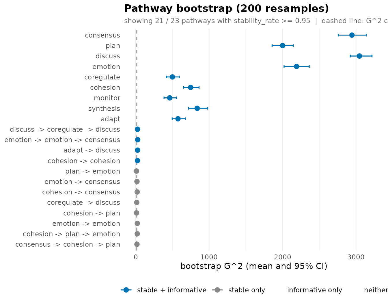
In the forest plot each bar is a 95% bootstrap interval on G-squared; the dashed line is the chi-square critical value. A bar entirely to the right is reproducibly informative; a bar straddling the line is not safe to claim.
9. Do high and low achievers regulate differently?
Fit one tree per group in a single call with
group =, then test where the groups diverge with a
permutation null. The grouping variable is an external student
attribute (Achiever), not derived from the actions
themselves – otherwise the comparison would be circular.
grp <- context_tree(group_regulation_long,
                    actor = "Actor", time = "Time", action = "Action",
                    group = "Achiever", max_depth = 2L, min_count = 10L)
cmp <- compare_groups(grp, iter = 199L, seed = 1L)
cmp$omnibus
#>         axis                 statistic    value p_value
#> 1 behavioral count-weighted JSD (bits) 1772.142   0.005
#> 2      usage                   sum G^2 1356.465   0.005
The omnibus table reports two axes. behavioral is
the count-weighted Jensen-Shannon divergence (bits) between the groups’
next-action distributions, summed over shared contexts – “given the same
history, do the groups do different things next?”.
usage is the summed G-squared homogeneity statistic –
“do they reach the same contexts at the same rates?”. Each
p_value comes from permuting the group labels.
plot_difference(grp, depth = 1L)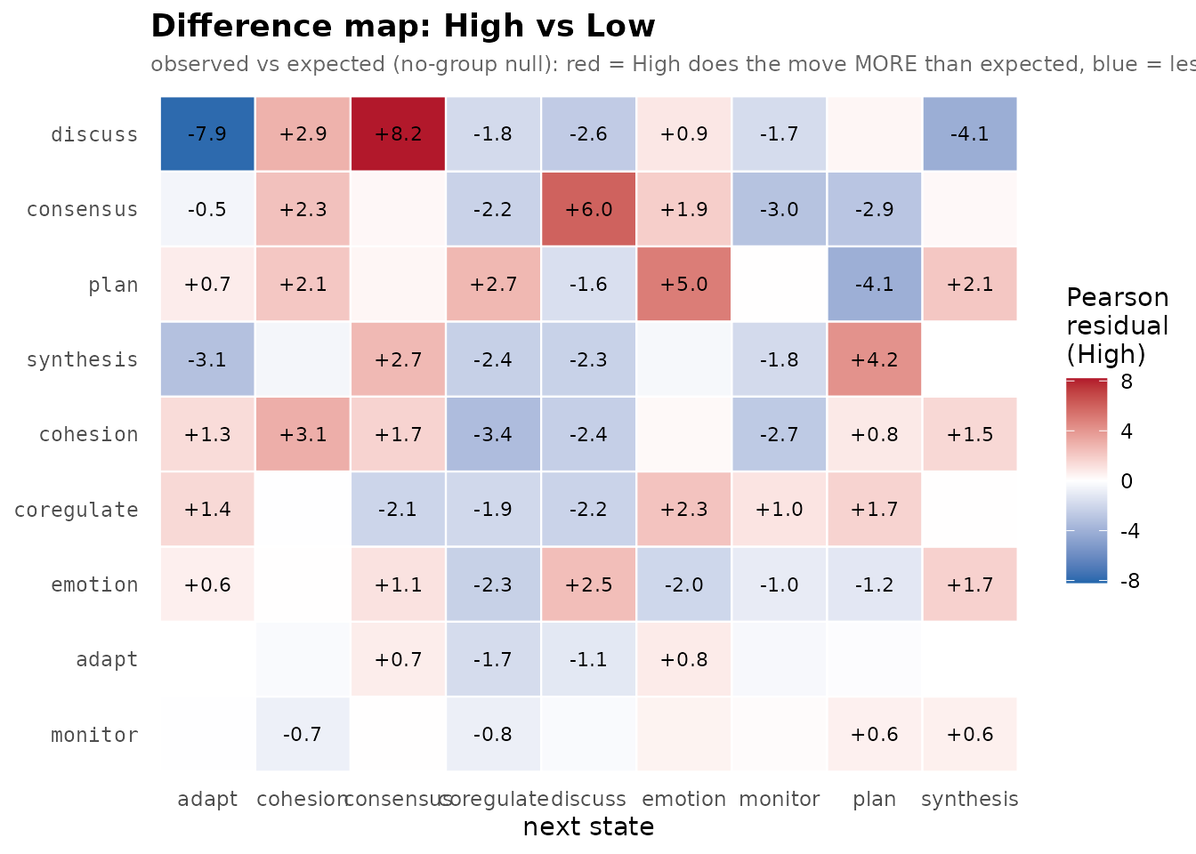
The per-context residual map shows where the groups differ:
red and blue cells are the contexts a high achiever and a low achiever
resolve toward different next actions. depth = 1L restricts
it to the single-action contexts so the rows stay readable; drop it (or
raise it) to inspect deeper histories.
Synthesis
Pulling the thread through every section:
-
The action alphabet is imbalanced – frequency is a
misleading lens and modal predictions are trivially
consensus/plan. - Memory is short – pruning collapses the tree to a small set of contexts, and held-out perplexity confirms the shallow model generalises.
- The insight is in the divergent, well-counted contexts – not the common ones, and not the spectacular low-count tail.
- Only the stable-and-informative pathways are claimable – the bootstrap is the trust filter between an eyeballed table and a finding.
- High and low achievers regulate measurably differently – the permutation test licenses the claim that the omnibus statistic is real, not a relabelling artefact.
Each claim is anchored to a function whose output you can re-run – the whole point of a pathway-centric, testable model.