Visual diagnostics for how a fitted tree scores held-out sequences,
built on score_positions():
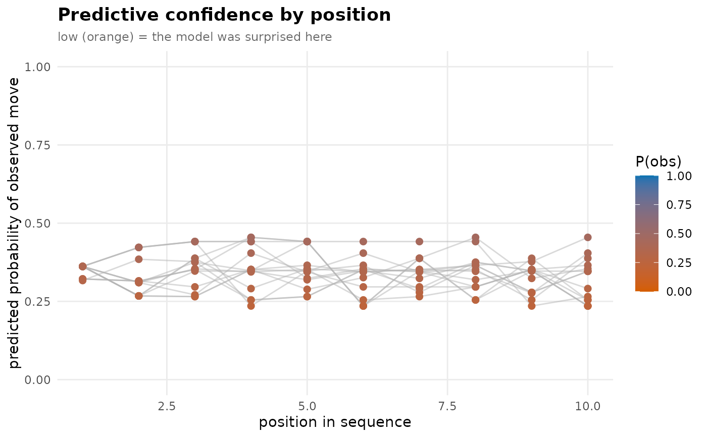
type = "position"predicted probability of the observed next state against position in the sequence — where the model is confident vs. surprised as a sequence unfolds.
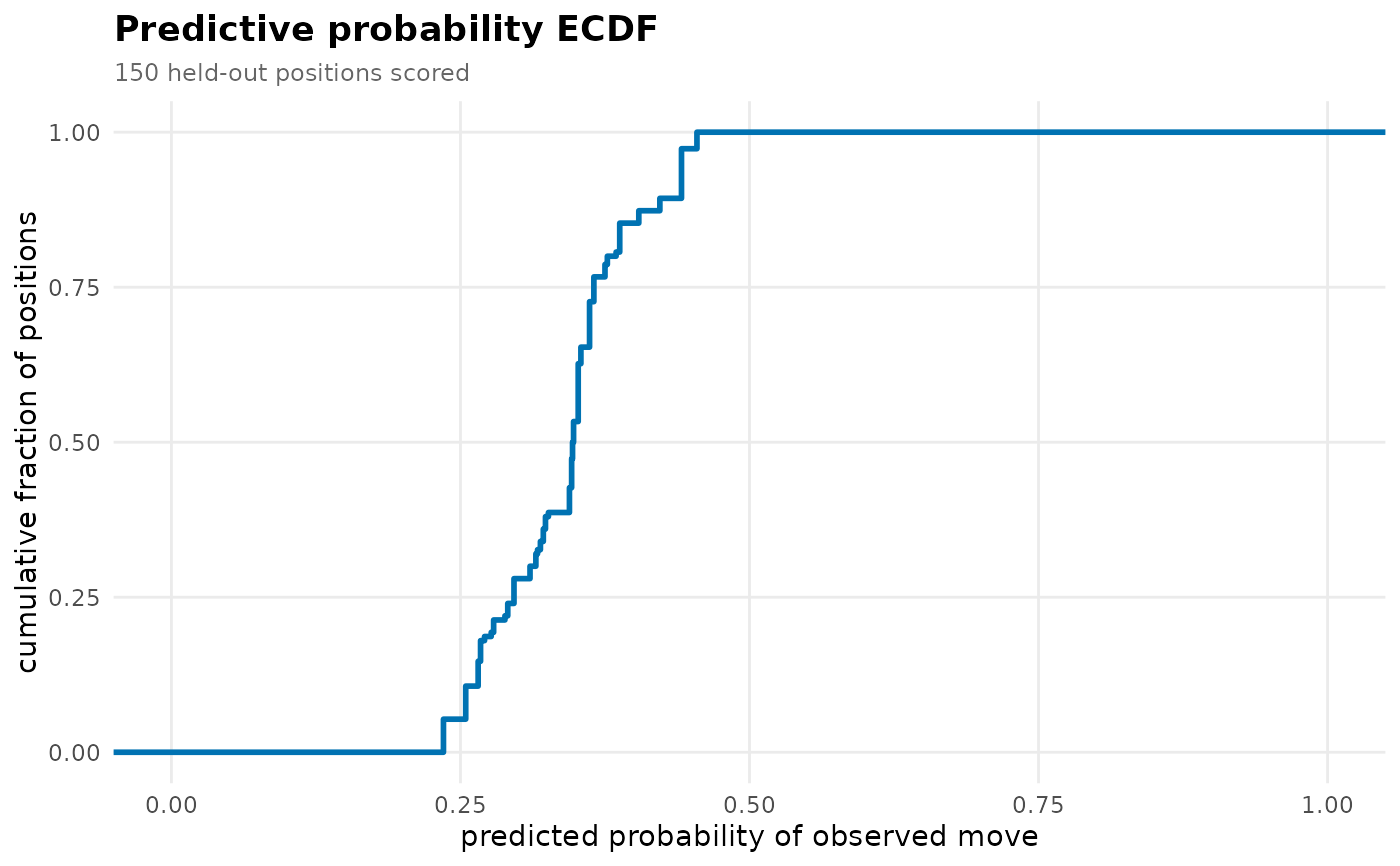
type = "ecdf"the empirical cumulative distribution of those predicted probabilities — a calibration-style view of how often the model assigns high vs. low probability to what actually happened.
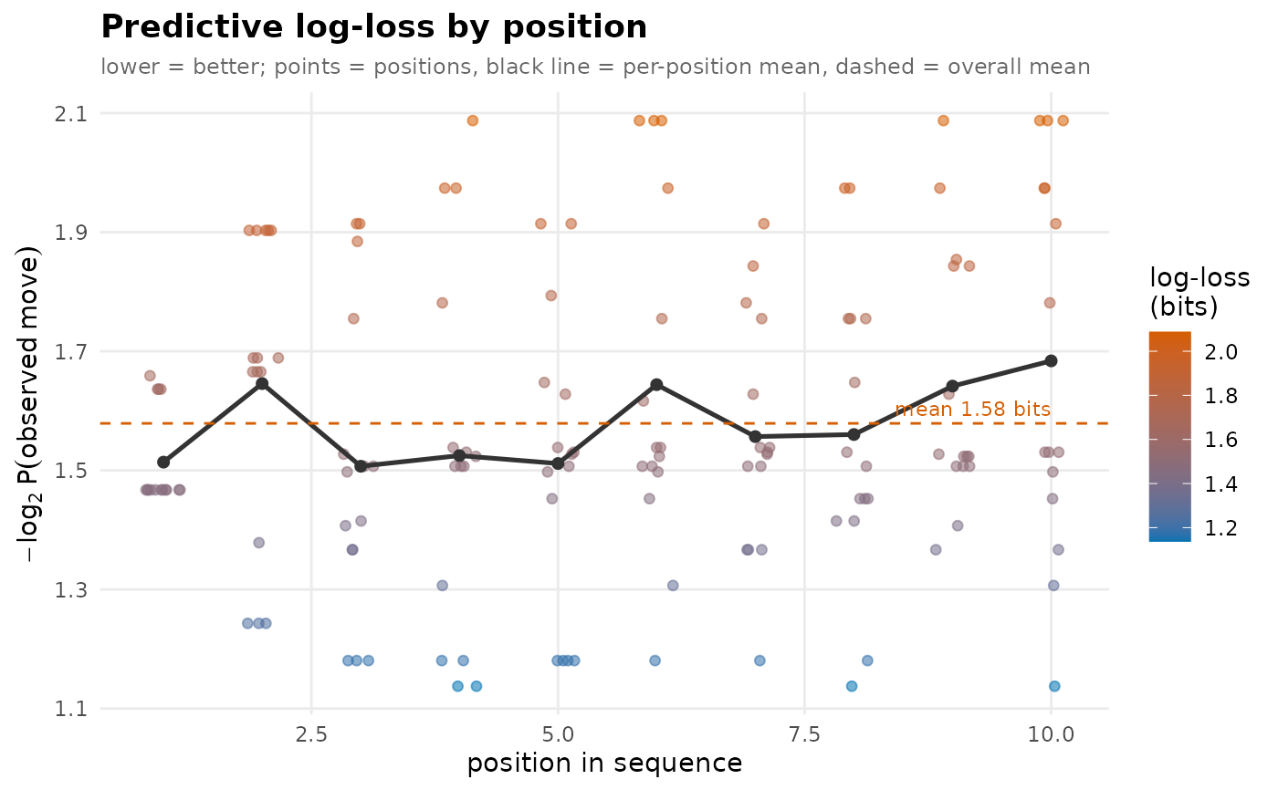
type = "logloss"the per-position log-loss \(-\log_2 P(\mathrm{observed})\) against position — a per-position log-loss view. Lower is better (0 = certain and correct); the dashed line is the mean log-loss over all scored positions.
Usage
plot_predictive(tree, newdata, type = c("position", "ecdf", "logloss"))Arguments
- tree
A
transitiontrees.- newdata
Held-out sequence data in any format accepted by
context_tree().- type
One of
"position"(default),"ecdf", or"logloss".
Examples
# \donttest{
fit <- replicate(60, sample(c("A", "B", "C"), 10, replace = TRUE),
simplify = FALSE)
tree <- context_tree(fit, max_depth = 2L)
new <- replicate(15, sample(c("A", "B", "C"), 10, replace = TRUE),
simplify = FALSE)
plot_predictive(tree, new, type = "position")
 plot_predictive(tree, new, type = "ecdf")
 plot_predictive(tree, new, type = "logloss")
 # }
# }