Visualizing bootstrap, centrality and difference results (base R)

Network diagnostics

Plotting networks and diagnostic results

psychnets provides a comprehensive set of visualization methods for estimated psychometric networks and their associated diagnostic analyses, facilitating both interpretation and statistical assessment. In addition to graphical displays, all estimation and diagnostic functions return tidy result objects that can be inspected programmatically, summarized numerically, or incorporated into downstream analytical workflows.

Psychometric networks are estimated from finite samples, and consequently every estimated edge weight, centrality measure, and derived statistic is subject to sampling variability. The diagnostic procedures implemented in psychnets quantify this uncertainty using non-parametric bootstrap resampling, case-dropping resampling, and permutation-based hypothesis testing. Each diagnostic returns a structured result object containing both the numerical results and the information required for graphical representation.

All graphical output is generated through dedicated plot() methods implemented for the corresponding result classes. These methods rely exclusively on the base R graphics and grDevices systems and therefore require no external visualization libraries. Throughout this tutorial, each figure is produced by fitting a network, applying a diagnostic procedure, and calling plot() on the returned object. The following sections describe the interpretation of the principal visualizations, including network plots, centrality measures, bootstrap confidence intervals, difference matrices, pairwise difference tests, case-dropping stability curves, and network comparison tests.

The data

The bundled SRL_GPT data hold responses from 300 learners on five self-regulated-learning constructs (CSU, IV, SE, SR, TA), each a continuous subscale score.

head(SRL_GPT)
#>        CSU       IV       SE       SR   TA
#> 1 5.307692 5.666667 5.777778 5.333333 4.00
#> 2 5.846154 6.444444 6.000000 5.777778 4.00
#> 3 6.615385 6.666667 6.222222 6.333333 3.25
#> 4 5.692308 6.555556 6.333333 5.555556 4.50
#> 5 4.384615 5.555556 4.888889 4.777778 4.00
#> 6 4.846154 5.444444 5.666667 5.111111 3.50

Estimate a network

ebic_glasso() estimates a Gaussian graphical model whose edges are partial correlations selected by the extended Bayesian information criterion. The fitted object is the input to every diagnostic below.

fit <- ebic_glasso(SRL_GPT)
fit
#> <psychnet> glasso network
#>   nodes: 5   edges: 10   (undirected)
#>   lambda: 0.00861   gamma: 0.5
#>   optimality (KKT residual): 2.21e-10

Centralities

net_centralities() computes node centrality measures from the fitted network and returns a tidy table with one row per node and one column per measure. Strength is the sum of absolute edge weights at a node, expected influence is the sum of signed edge weights, and betweenness counts the weighted shortest paths that pass through a node.

ct <- net_centralities(fit, measures = c("strength", "expected_influence", "betweenness"))
ct
#>   node  strength expected_influence betweenness
#> 1  CSU 1.1984512         1.19845117   0.3333333
#> 2   IV 1.0012765         1.00127649   0.0000000
#> 3   SE 0.8492185         0.84921854   0.0000000
#> 4   SR 1.2314317         0.53172852   1.0000000
#> 5   TA 0.6082238        -0.09147935   0.0000000

plot() for a psychnet_centrality table draws one panel per measure. Under the default type = "bar", each panel is a horizontal lollipop chart whose nodes are sorted by their value, so the most central node sits at the top of the panel and the length of each segment reads directly as the centrality value.

plot(ct)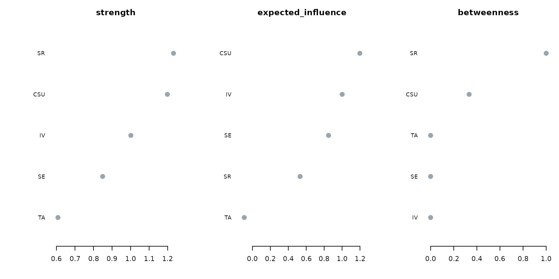

Under type = "line", plot() draws the faceted centrality profile. The nodes share a single vertical order across all panels, set by their mean standardized centrality, and each panel keeps its own horizontal axis. A node that sits high in every panel is central on every measure; a node whose position shifts between panels is central on one measure and peripheral on another.

plot(ct, type = "line")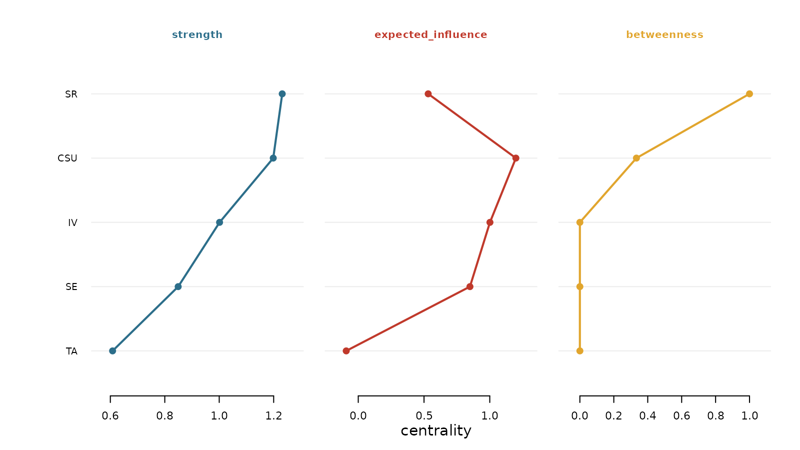

The scale argument controls the per-panel transform in the line view. The default "raw" keeps each panel on its own axis of centrality values, "z" centres each measure at its mean and scales it to unit standard deviation, and "relative" maps each measure to the interval from zero to one.

plot(ct, type = "line", scale = "z")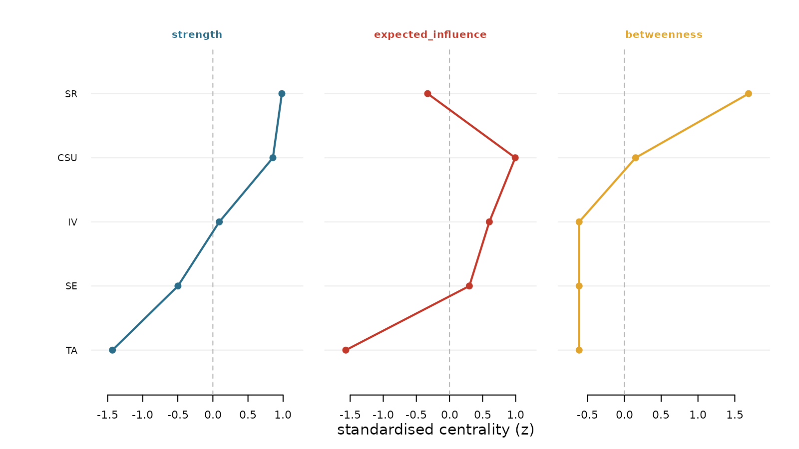

Bootstrap accuracy

net_boot() resamples the rows of the data with replacement, refits the network on each resample, and records the distribution of every edge weight and every centrality value across resamples. The percentile confidence interval of each quantity is the reported measure of its sampling accuracy.

set.seed(1)
bs <- net_boot(SRL_GPT, method = "glasso", n_boot = 250, cores = 1)

plot() for a psychnet_bootstrap object defaults to type = "edges", the edge-accuracy plot. Each row is an edge, sorted by its observed weight; the point is the observed weight and the segment is its bootstrap confidence interval. An edge whose interval excludes zero is drawn in the emphasis colour, which reports that the edge is present across resamples; an edge whose interval crosses zero is muted.

plot(bs)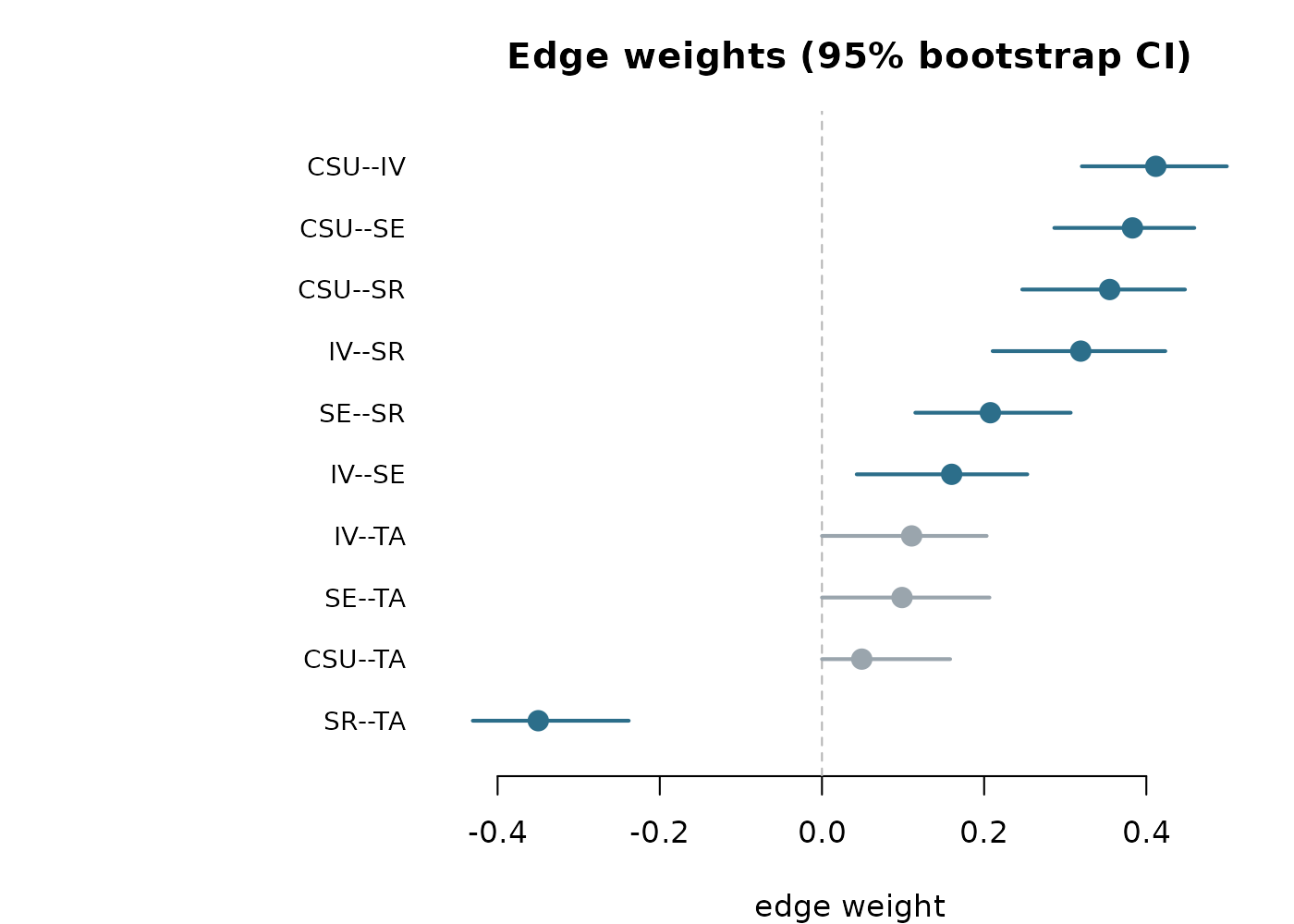

Under type = "centrality", plot() draws the bootstrapped centrality intervals, one sorted panel per measure. A node whose interval is wide relative to the spread across nodes is estimated with low precision, so its rank among the nodes is uncertain.

plot(bs, type = "centrality")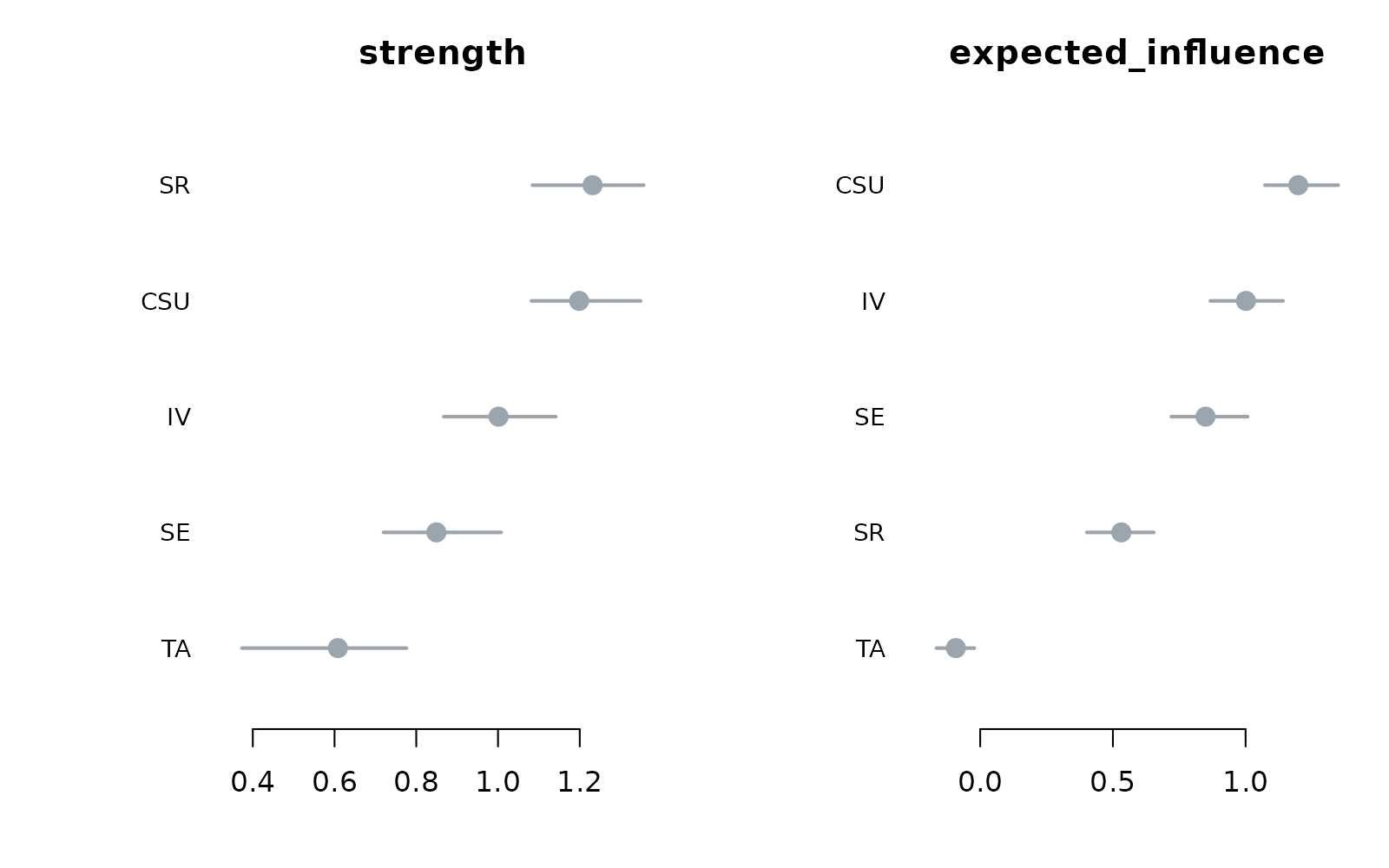

Under type = "edge_diff" and type = "centrality_diff", plot() draws the difference “significance box” matrix. The items sit on both axes, ordered by their observed value from high to low. The diagonal carries the observed value, shaded by its magnitude. An off-diagonal cell is filled when that pair of items differs across the bootstrap, coloured red when the row item is larger than the column item and blue when it is smaller, and it is left faint when the pair does not differ. The stars report the difference p-value.

plot(bs, type = "edge_diff")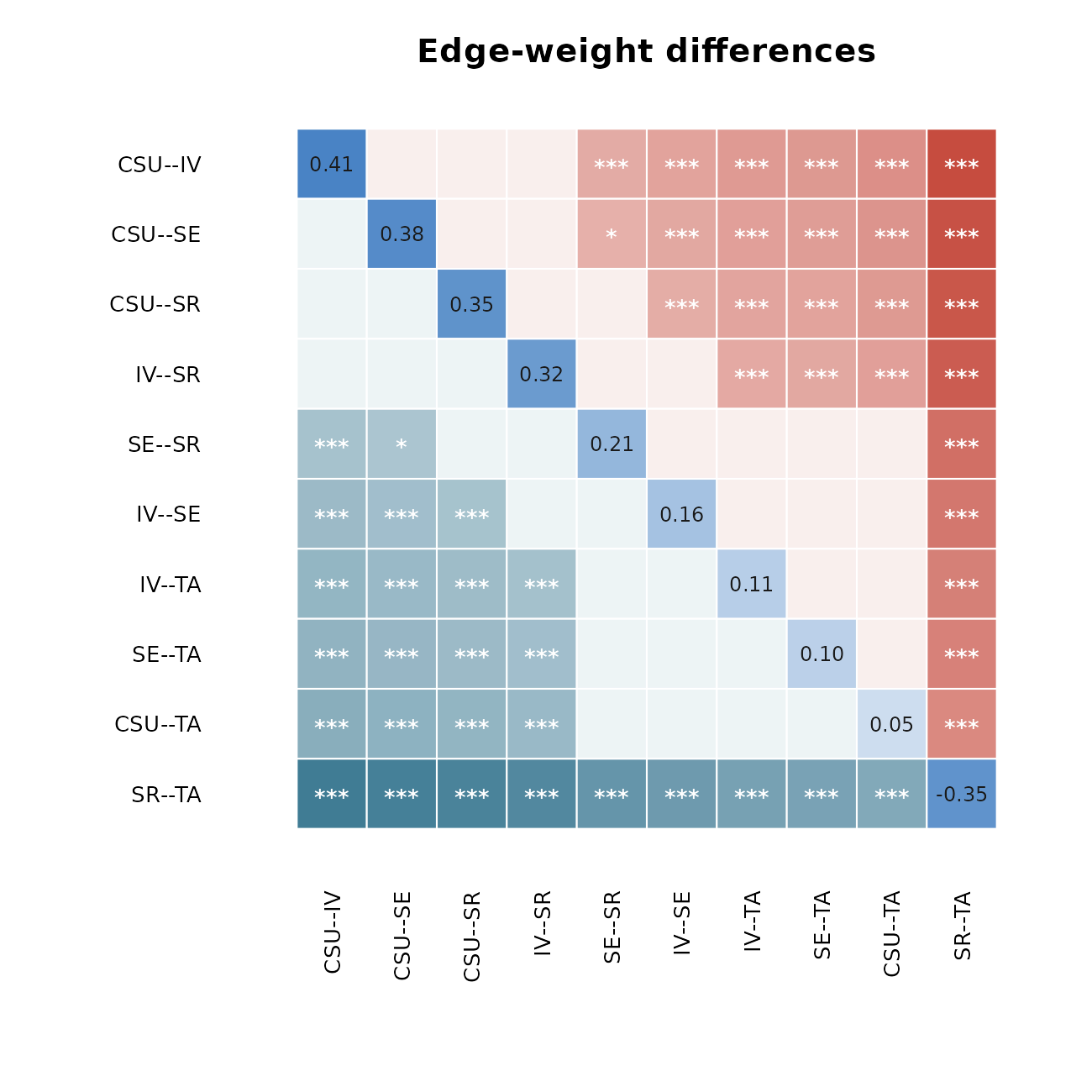

plot(bs, type = "centrality_diff", measure = "strength")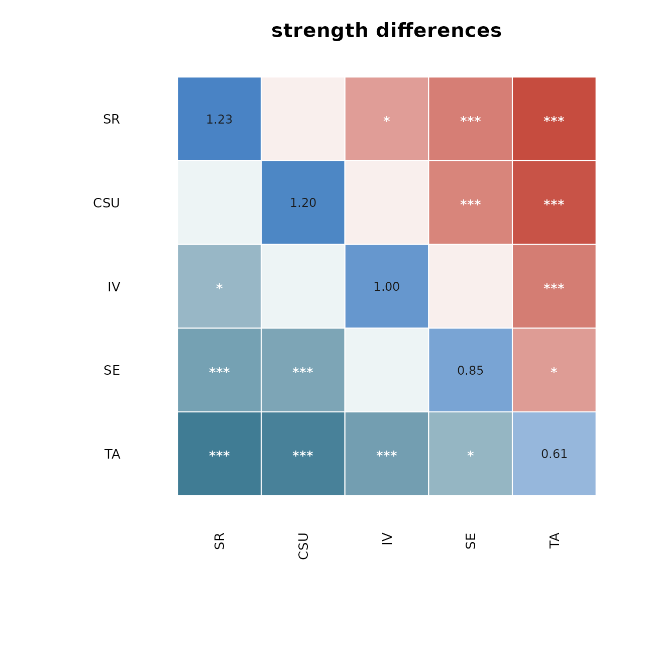

Difference test

difference_test() reads the retained bootstrap draws and returns a tidy table of pairwise differences, with columns item1, item2, the two observed values, the observed difference obs_diff, its interval lower and upper, the p_value, and a significant flag set when the interval excludes zero.

dt <- difference_test(bs, type = "strength")
head(dt)
#>   item1 item2    value1    value2    obs_diff       lower       upper p_value
#> 1   CSU    IV 1.1984512 1.0012765  0.19717467 -0.01516075  0.43862886   0.080
#> 2   CSU    SE 1.1984512 0.8492185  0.34923263  0.12605796  0.63527516   0.000
#> 3    IV    SE 1.0012765 0.8492185  0.15205795 -0.09197932  0.36727209   0.208
#> 4   CSU    SR 1.1984512 1.2314317 -0.03298049 -0.21134715  0.18144546   0.712
#> 5    IV    SR 1.0012765 1.2314317 -0.23015517 -0.41550510 -0.04600301   0.024
#> 6    SE    SR 0.8492185 1.2314317 -0.38221312 -0.54711539 -0.20825524   0.000
#>   significant
#> 1       FALSE
#> 2        TRUE
#> 3       FALSE
#> 4       FALSE
#> 5        TRUE
#> 6        TRUE

plot() for a psychnet_difference table has two styles. The default style = "box" draws the same significance-box matrix as above, which reads which pairs differ.

plot(dt)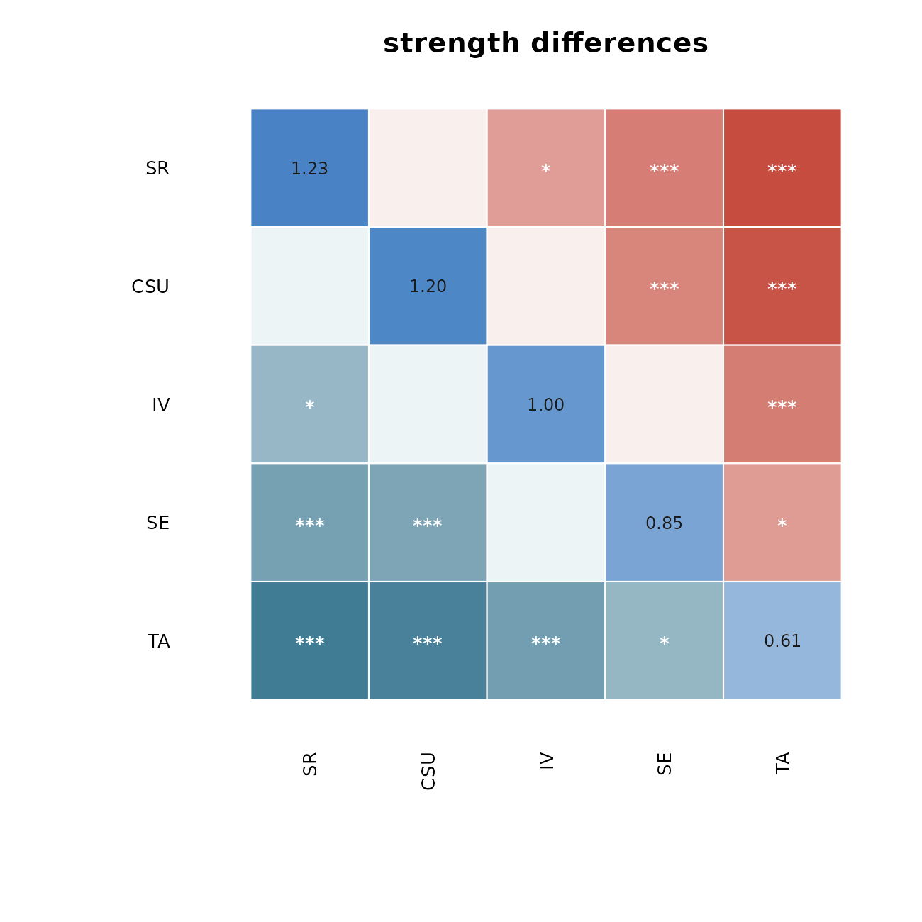

Under style = "forest", plot() draws a forest plot with one row per pair. The point is the observed difference, the segment is its confidence interval, the dashed line marks zero, and a pair whose interval excludes zero is emphasised. This view reads how large each difference is together with its uncertainty.

plot(dt, style = "forest")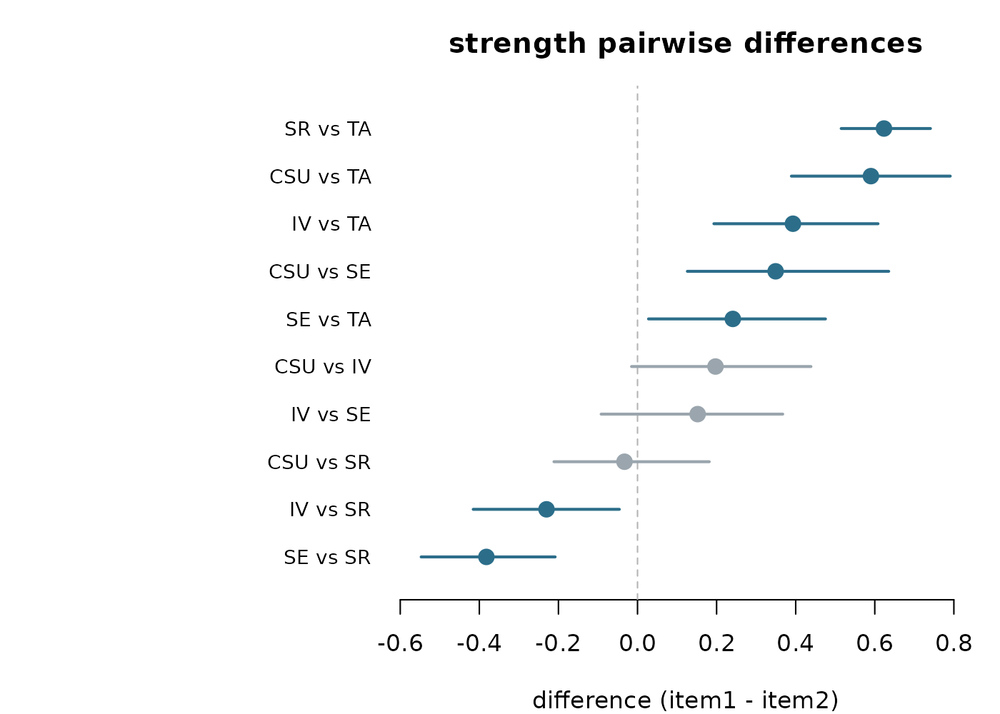

Case-dropping stability

net_stability() drops an increasing fraction of the cases, refits the network on each subset, and correlates the subset centralities with the full-sample centralities. The case-dropping (CS) coefficient is the largest drop proportion at which the correlation stays above the acceptance threshold with the stated certainty.

st <- net_stability(SRL_GPT, method = "glasso",
                    drop_prop = seq(0.1, 0.8, 0.1), iter = 25)

plot() for a psychnet_stability object draws the stability curves. The horizontal axis is the proportion of cases dropped and the vertical axis is the mean correlation with the full sample. Each measure is a line with a band of plus or minus one standard deviation, the dashed line is the acceptance threshold, and the legend reports the CS-coefficient for each measure. A curve that stays above the threshold as more cases are dropped indicates a stable centrality ordering.

plot(st)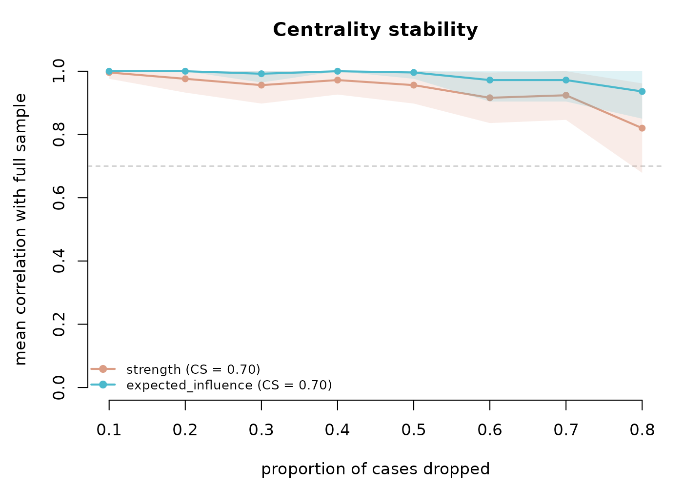

Network comparison test

net_compare() compares two networks by permutation. It repeatedly reassigns the pooled cases to two groups at random, recomputes the test statistic on each permutation, and builds the distribution of that statistic expected when the two networks do not differ. The global strength statistic (M) is the difference in summed absolute edge weights, and the structure statistic (S) is the maximum absolute edge difference.

cmp <- net_compare(SRL_GPT, SRL_Claude, iter = 250)

plot() for a psychnet_nct object defaults to type = "strength", the permutation null for M. The histogram is the null distribution, the red line marks the observed value, and the title reports the permutation p-value. An observed value in the tail of the null provides evidence that the two networks differ in global strength.

plot(cmp)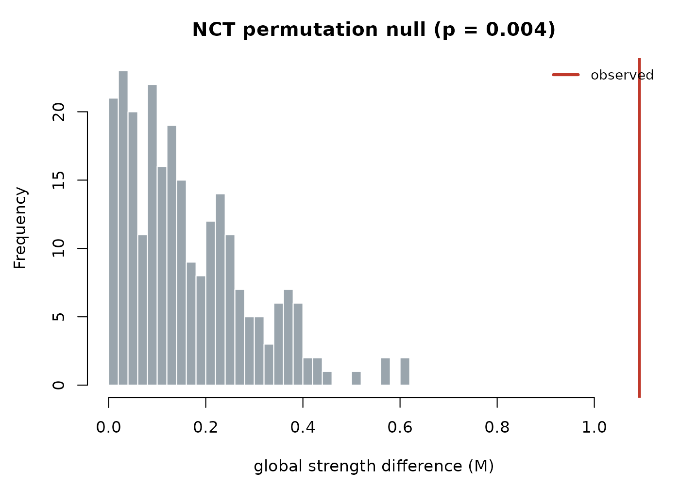

Under type = "structure", plot() draws the same null for the maximum edge-difference statistic S.

plot(cmp, type = "structure")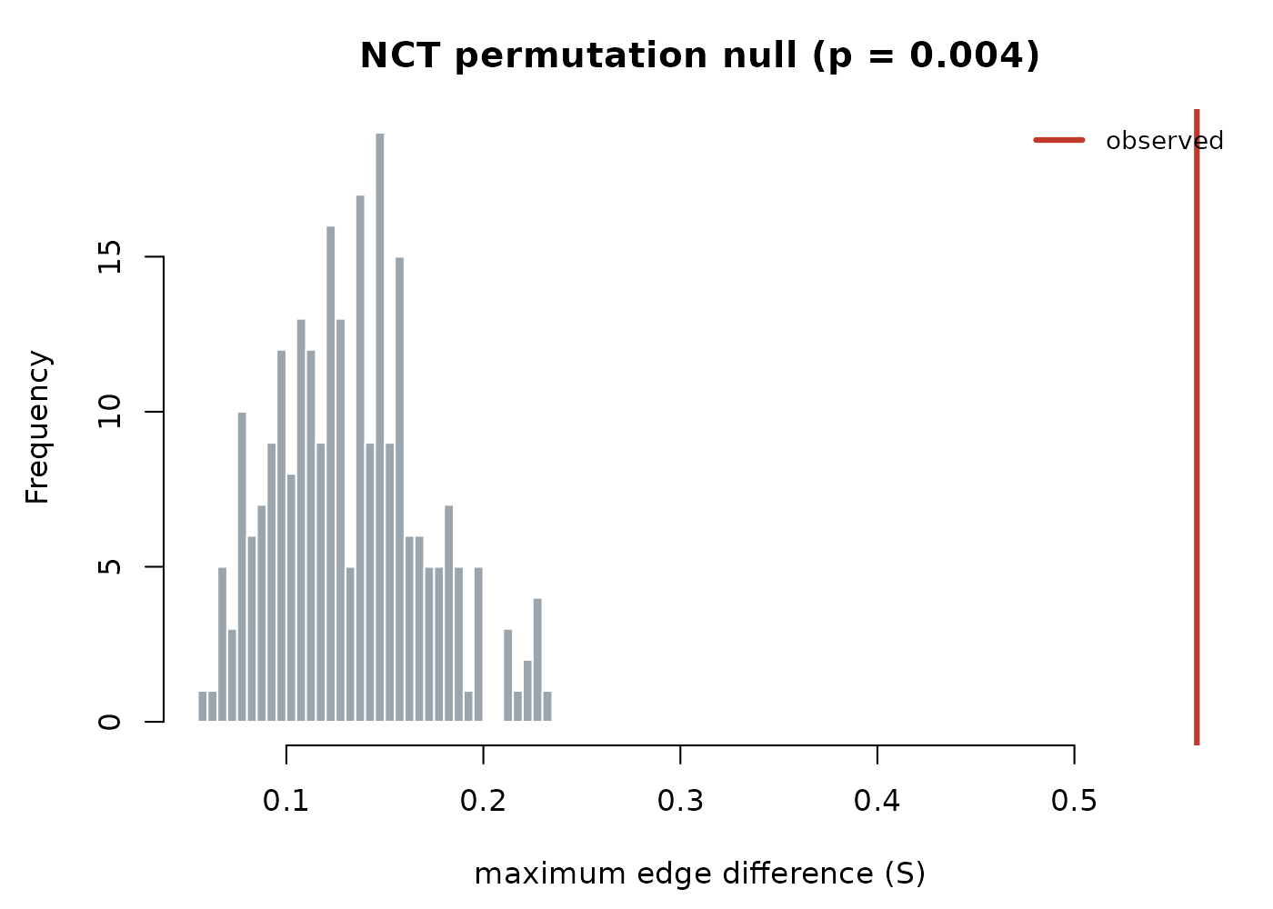

Under type = "edges", plot() draws the observed absolute difference of each edge as a horizontal bar, coloured by whether that edge differs significantly at the level set by alpha. The title reports how many edges reach significance.

plot(cmp, type = "edges")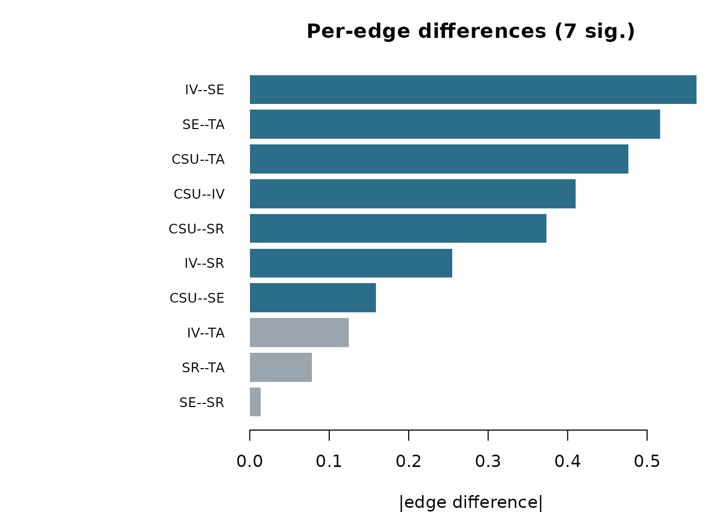

The plot methods at a glance

Result object (verb)	`plot()` options
`net_centralities()`	`type = "bar"` / `"line"`; `scale = "raw"` / `"z"` / `"relative"`
`net_boot()`	`type = "edges"` / `"centrality"` / `"edge_diff"` / `"centrality_diff"` / `"predictability"`
`difference_test()`	`style = "box"` / `"forest"`
`net_stability()`	one figure
`net_compare()`	`type = "strength"` / `"structure"` / `"edges"`

Each figure above is drawn with base R alone. For the estimated network itself, plot(fit) delegates to cograph::splot(), covered in the companion vignette Visualizing networks with cograph.

Mohammed Saqr