Gaussian graphical models: estimation and interpretation

What a Gaussian graphical model is

A Gaussian graphical model represents the conditional dependence structure of a set of continuous variables. Each node corresponds to an observed variable, and each edge represents the partial correlation between two variables after conditioning on every other variable in the network. The graph is undirected because partial correlations are symmetric; the association between variables (i) and (j) is identical to that between (j) and (i).

The objective of a Gaussian graphical model is to determine whether two variables remain associated after the influence of all other measured variables has been removed. Consider a network containing motivation, academic achievement, prior achievement, study effort, self-efficacy, and test anxiety. An edge between motivation and academic achievement indicates that these variables remain conditionally associated after accounting for prior achievement, study effort, self-efficacy, and test anxiety. The edge therefore represents the component of their relationship that cannot be explained by the remaining variables included in the model.

Conversely, the absence of an edge indicates that the model does not retain a unique conditional association between the two variables after adjustment for the remaining variables. Their marginal correlation may nevertheless be substantial. For example, the observed association between motivation and academic achievement may be explained through their relationships with study effort, self-efficacy, or prior achievement. Gaussian graphical models distinguish these indirect pathways from associations that remain after statistical adjustment for all other variables.

During estimation, weak conditional associations that are consistent with sampling variability are removed, producing a sparse representation of the conditional dependence structure. Consequently, a missing edge should not be interpreted as evidence that two variables are universally unrelated, but rather that the observed data do not provide sufficient evidence for a direct conditional association under the fitted model. Likewise, the presence of an edge indicates statistical dependence conditional on the measured variables and should not be interpreted as evidence of a causal relationship.

In psychnets, Gaussian graphical models are implemented as a clean-room reimplementation in base R. Both the statistical estimator and the numerical optimization algorithm are implemented directly in R from first principles, without invoking compiled Fortran or C/C++ optimization libraries or external estimation packages. This implementation provides complete transparency of the estimation procedure while reproducing the established Gaussian graphical model methodology.

The data

The worked example uses SRL_GPT, a data frame supplied with psychnets. It contains 300 observations on five construct scores from a self-regulated learning questionnaire. Cognitive strategy use (CSU), intrinsic value (IV), self-efficacy (SE), self-regulation (SR), and test anxiety (TA) are means of item responses recorded on a 1 to 7 scale.

head(SRL_GPT)
#>        CSU       IV       SE       SR   TA
#> 1 5.307692 5.666667 5.777778 5.333333 4.00
#> 2 5.846154 6.444444 6.000000 5.777778 4.00
#> 3 6.615385 6.666667 6.222222 6.333333 3.25
#> 4 5.692308 6.555556 6.333333 5.555556 4.50
#> 5 4.384615 5.555556 4.888889 4.777778 4.00
#> 6 4.846154 5.444444 5.666667 5.111111 3.50

Rows are observations and columns are network nodes. The analysis treats the five scale scores as continuous variables. This treatment is most defensible when each score aggregates several items and has enough distinct values to approximate a continuous distribution. Item-level ordinal data may require an ordinal correlation estimator, discussed under sensitivity analysis.

Before fitting a network, a scientific analysis should also examine missingness, univariate distributions, unusual observations, and the effective sample size. The current data are complete. The default estimator therefore uses the same 300 observations for every pairwise correlation.

Fitting the network with psychnet()

psychnet() estimates a network from a numeric table and returns a fitted psychnet object. The argument method = "glasso" requests an EBIC-regularized Gaussian graphical model. The default settings use Pearson correlations, pairwise-complete handling of missing values, $\gamma = 0.5$, and the package’s native graphical-lasso solver.

net <- psychnet(data = SRL_GPT, method = "glasso")
net
#> <psychnet> glasso network
#>   nodes: 5   edges: 10   (undirected)
#>   lambda: 0.00861   gamma: 0.5
#>   optimality (KKT residual): 2.21e-10

The printed object reports 5 nodes and 10 retained edges. The selected penalty is $\lambda = 0.00861$ at $\gamma = 0.5$. All possible pairs are retained in this small example, although several estimated edges are weak. The selected penalty and the observed data determine the degree of sparsity in each fitted network.

Inspecting edges with summary()

summary() prints the fitted model and returns its edge table invisibly. The table contains the columns from, to, and weight. Each row identifies a retained pair of nodes and its estimated partial correlation.

summary(net)
#> <psychnet> glasso network
#>   nodes: 5   edges: 10   (undirected)
#>   lambda: 0.00861   gamma: 0.5
#>   optimality (KKT residual): 2.21e-10
#>   edge weight: range [-0.350, 0.412], mean 0.174

The edge weights range from -0.350 to 0.412, with a mean of 0.174 across the 10 retained edges. The positive CSU-IV edge is the largest positive conditional association ($r = 0.412$). Cognitive strategy use and intrinsic value remain positively associated after adjustment for self-efficacy, self-regulation, and test anxiety.

The SR-TA edge is negative ($r = -0.350$). Higher self-regulation is associated with lower test anxiety among observations with comparable values on the other three constructs. The edges from TA to CSU ($r = 0.049$), SE ($r = 0.099$), and IV ($r = 0.111$) are small. Their magnitudes support only cautious substantive interpretation. None of these conditional associations identifies a causal effect.

Checking numerical optimality with certificate()

certificate() reports how closely a fitted estimator satisfies the defining conditions of its optimization problem. For a graphical-lasso fit, the returned data frame has the columns method, certificate, kind, and certified. The certificate value is the maximum violation of the Karush-Kuhn-Tucker (KKT) stationarity conditions. The kind value is "kkt", and certified records whether the residual is at or below the requested tolerance of $10^{-6}$ by default.

certificate(net)
#>   method  certificate kind certified
#> 1 glasso 2.213401e-10  kkt      TRUE

The KKT residual is $2.21 \times 10^{-10}$ and certified is TRUE. This residual is close to machine precision. It indicates that the estimated precision matrix satisfies the first-order conditions of the selected convex objective to numerical precision. The certificate assesses numerical optimization. It does not assess the Gaussian assumption, the substantive validity of the variables, sampling uncertainty, or causal identification.

Describing node position with net_centralities()

net_centralities() computes node-level summaries from the fitted weighted graph. Its default return is a tidy data frame with the columns node, strength, and expected_influence. Strength is the sum of the absolute edge weights incident on a node. Expected influence is the sum of the signed edge weights, so negative and positive relations can offset one another.

net_centralities(net)
#>   node  strength expected_influence
#> 1  CSU 1.1984512         1.19845117
#> 2   IV 1.0012765         1.00127649
#> 3   SE 0.8492185         0.84921854
#> 4   SR 1.2314317         0.53172852
#> 5   TA 0.6082238        -0.09147935

Self-regulation has the largest strength (1.231), followed by cognitive strategy use (1.198). Self-regulation combines several positive connections with the negative connection to test anxiety. Its expected influence is therefore 0.532, which is lower than its strength. Cognitive strategy use has only positive estimated edges, so its strength and expected influence are both 1.198.

Test anxiety has strength 0.608 and expected influence -0.091. Its negative edge with self-regulation offsets its three small positive edges. This example shows why the two indices answer different questions. Strength quantifies total absolute connection, whereas expected influence retains the direction of each relation. Centrality is a descriptive property of the estimated graph. A high value does not identify a variable as a cause or an intervention target.

Quantifying node predictability with net_predict()

net_predict() reports how well every node is predicted by the other nodes in a fitted network. For a Gaussian graphical model, it computes the proportion of variance explained, $R^2$, directly from the precision and covariance matrices. The returned data frame has the columns node, type, metric, predictability, and accuracy. The Gaussian rows use type = "gaussian", metric = "R2", and accuracy = NA because classification accuracy does not apply to continuous nodes.

net_predict(net)
#>   node     type metric predictability accuracy
#> 1  CSU gaussian     R2      0.8217840       NA
#> 2   IV gaussian     R2      0.7690346       NA
#> 3   SE gaussian     R2      0.7142811       NA
#> 4   SR gaussian     R2      0.7786477       NA
#> 5   TA gaussian     R2      0.1421163       NA

Cognitive strategy use has the largest predictability, with $R^2 = 0.822$. Self-regulation ($R^2 = 0.779$), intrinsic value ($R^2 = 0.769$), and self-efficacy ($R^2 = 0.714$) are also strongly explained by their remaining nodes in this fitted model. Test anxiety has $R^2 = 0.142$, so the other four constructs account for a much smaller proportion of its variance.

Predictability complements centrality. Centrality summarizes how a node is connected, while predictability quantifies how much of its variance is accounted for by the other nodes. Predictability remains an in-sample model quantity in this analysis. It should not be read as out-of-sample predictive performance without a separate validation design.

Visualizing the fitted network with cograph::splot()

cograph::splot() draws the fitted object as a network when the optional cograph package is available. The argument psych_styling = TRUE uses green edges for positive weights, red edges for negative weights, and node rings for the stored predictability values.

cograph::splot(net, psych_styling = TRUE)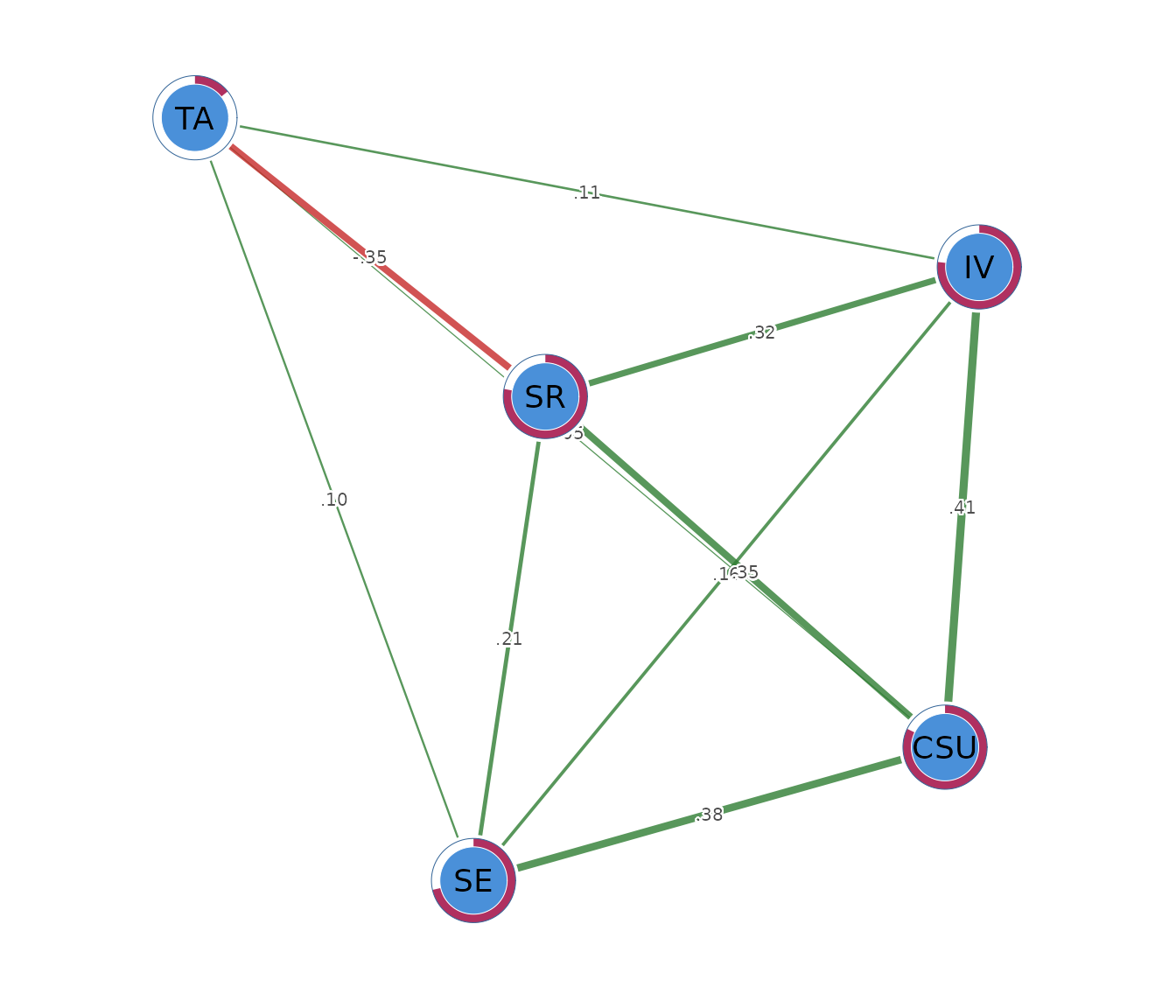

The figure is a compact representation of the edge table. Edge colour encodes sign and edge width encodes magnitude. Node position is determined by a layout algorithm and has no direct statistical scale. Visual distance between two nodes must therefore not be interpreted as an estimated association. Numerical interpretation should return to the edge table and node-level summaries.

Sensitivity to the correlation estimator

Analytic choices can affect weak edges. A sensitivity analysis changes one choice at a time and compares the resulting model with the primary fit. psychnet() accepts cor_method = "spearman" for a rank-based analysis. Spearman correlations reduce sensitivity to monotone transformations and extreme values, although they answer a rank-association version of the research question.

spearman_net <- psychnet(data = SRL_GPT, method = "glasso", cor_method = "spearman")
spearman_net
#> <psychnet> glasso network
#>   nodes: 5   edges: 9   (undirected)
#>   lambda: 0.01882   gamma: 0.5
#>   optimality (KKT residual): 2.67e-10

summary(spearman_net)
#> <psychnet> glasso network
#>   nodes: 5   edges: 9   (undirected)
#>   lambda: 0.01882   gamma: 0.5
#>   optimality (KKT residual): 2.67e-10
#>   edge weight: range [-0.237, 0.424], mean 0.192

The Spearman analysis retains 9 edges and selects $\lambda = 0.01882$. The main pattern remains: the four learning constructs are positively connected and the SR-TA edge is negative. The weak CSU-TA edge is absent, and the SR-TA estimate changes from -0.350 to -0.237. The persistence of the main pattern provides evidence that its qualitative interpretation is not specific to Pearson correlations. The changes in weaker edges indicate sensitivity in that part of the graph.

For item-level ordinal variables, cor_method = "auto" can estimate polychoric or polyserial associations where appropriate. The measurement scale should determine this choice before the network results are examined.

Applying a substantive edge threshold

psychnet() can apply an absolute post-estimation threshold through its threshold argument. A threshold is a reporting or sparsification choice. It does not change the penalty selected by EBIC, and it should be justified before examining the final graph.

threshold_net <- psychnet(data = SRL_GPT, method = "glasso", threshold = 0.1)
threshold_net
#> <psychnet> glasso network
#>   nodes: 5   edges: 8   (undirected)
#>   lambda: 0.00861   gamma: 0.5
#>   optimality (KKT residual): 2.21e-10

summary(threshold_net)
#> <psychnet> glasso network
#>   nodes: 5   edges: 8   (undirected)
#>   lambda: 0.00861   gamma: 0.5
#>   optimality (KKT residual): 2.21e-10
#>   edge weight: range [-0.350, 0.412], mean 0.200

At a threshold of 0.10, the graph contains 8 edges. The CSU-TA estimate (0.049) and the SE-TA estimate (0.099) are removed. The selected penalty and KKT residual are unchanged because thresholding occurs after estimation. A threshold can make a graph easier to read, but it must not be presented as a model-selection result from EBIC.

A nonparanormal sensitivity model

The Gaussian graphical model assumes joint normality for its exact probabilistic interpretation. psychnet() fits a rank-based nonparanormal model with method = "huge". This method estimates monotone marginal transformations and then applies the same EBIC graphical-lasso procedure to the transformed correlation matrix. Its purpose is to relax strict marginal normality while retaining a Gaussian conditional-dependence model on the transformed scale.

npn_net <- psychnet(data = SRL_GPT, method = "huge")
npn_net
#> <psychnet> huge network
#>   nodes: 5   edges: 10   (undirected)
#>   lambda: 0.008559   gamma: 0.5
#>   optimality (KKT residual): 2.47e-10

summary(npn_net)
#> <psychnet> huge network
#>   nodes: 5   edges: 10   (undirected)
#>   lambda: 0.008559   gamma: 0.5
#>   optimality (KKT residual): 2.47e-10
#>   edge weight: range [-0.343, 0.426], mean 0.172

The nonparanormal model retains all 10 edges. Its weights range from -0.343 to 0.426. The positive cluster among the four learning constructs and the negative SR-TA edge remain. The weakest CSU-TA edge decreases from 0.049 to 0.024, which again marks this edge as sensitive to the correlation model.

certificate(npn_net)
#>   method  certificate kind certified
#> 1   huge 2.471425e-10  kkt      TRUE

The KKT residual is $2.47 \times 10^{-10}$ and certified is TRUE. The optimization therefore satisfies its first-order conditions to numerical precision on the transformed correlation matrix. This result checks the solver, while the scientific adequacy of the nonparanormal model remains a modeling judgment.

Reporting the analysis

A complete report should identify the variables and their measurement scale, the sample size, the correlation estimator, the missing-data procedure, the network estimator, the EBIC value of $\gamma$, and any post-estimation threshold. It should report the edge weights numerically and distinguish conditional association from causation. Centrality and predictability should be defined before their values are interpreted.

The present analysis used Pearson correlations and an EBIC graphical lasso with $\gamma = 0.5$ on 300 complete observations. The selected model had 5 nodes, 10 edges, and $\lambda = 0.00861$. Its KKT residual was $2.21 \times 10^{-10}$. The largest positive edge joined cognitive strategy use and intrinsic value ($r = 0.412$), and the largest negative edge joined self-regulation and test anxiety ($r = -0.350$). Rank-based and nonparanormal sensitivity models preserved the main qualitative pattern but changed some weak edges.

Why the model removes weak connections

The graphical lasso filters small connections so that the fitted network focuses on associations with enough unique information to be retained. This filtering is useful because a sample can contain many negligible correlations produced by ordinary sampling variation. Keeping every one of them would make the network harder to read and could give weak, noisy connections more attention than their magnitudes justify.

The amount of filtering is selected from the data. psychnets fits networks across a sequence of penalty values and uses the extended Bayesian information criterion (EBIC) to balance fit with the number of retained edges. The hyperparameter $\gamma$ controls how strongly EBIC favours a simpler network. Larger values generally retain fewer edges.

This procedure explains how the graph was simplified. It does not make the retained edges causal, and it does not show that every removed edge is exactly zero in the population. Weak edges may change across samples or analytic choices, which is why the Spearman and nonparanormal examples above are useful.

Mathematical foundations

This section states the model, estimator, selection criterion, and numerical diagnostic precisely. The worked example can be understood without these derivations.

Precision matrix and conditional independence

Let $\mathbf{X} = (X_1, \ldots, X_p)^\mathsf{T}$ follow a multivariate normal distribution with mean vector $\boldsymbol{\mu}$ and positive-definite covariance matrix $\boldsymbol{\Sigma}$. The precision matrix is $\mathbf{K} = \boldsymbol{\Sigma}^{-1}$. For distinct nodes $i$ and $j$,

$$K_{ij} = 0 \quad \Longleftrightarrow \quad X_i \perp\!\!\!\perp X_j \mid \mathbf{X}_{\setminus\{i,j\}}.$$

Zeros in the precision matrix therefore define the missing edges of the population graph. The partial correlation associated with a retained edge is

$$\rho_{ij \cdot \mathrm{rest}} = -\frac{K_{ij}}{\sqrt{K_{ii}K_{jj}}}.$$

This standardization places conditional associations on the correlation scale, from -1 to 1.

Penalized likelihood

Let $\mathbf{S}$ be the sample covariance or correlation matrix. The graphical lasso estimates a positive-definite precision matrix by minimizing

$$\widehat{\mathbf{K}} = \underset{\mathbf{K} \succ 0}{\operatorname{argmin}} \left\{ -\log\det(\mathbf{K}) + \operatorname{tr}(\mathbf{S}\mathbf{K}) + \lambda \sum_{i \ne j}|K_{ij}| \right\}.$$

The tuning parameter $\lambda \geq 0$ controls the amount of regularization. Larger values impose more shrinkage on off-diagonal precision entries and usually produce fewer edges. The objective is strictly convex over the cone of positive-definite matrices, so its minimizer is unique.

EBIC model selection

For each candidate value of $\lambda$, the fitted graph has a Gaussian log-likelihood $\ell(\widehat{\mathbf{K}})$ and $E$ retained edges. The EBIC is

$$\operatorname{EBIC}_{\gamma} = -2\ell(\widehat{\mathbf{K}}) + E\log(n) + 4E\gamma\log(p),$$

where $n$ is the sample size, $p$ is the number of nodes, and $\gamma$ controls the additional graph-complexity penalty. psychnets evaluates a logarithmically spaced path of candidate penalties and selects the value with the smallest EBIC. The selected penalty is then refitted at a tighter numerical tolerance.

KKT optimality conditions

Write $\mathbf{W} = \widehat{\mathbf{K}}^{-1}$. At the optimum, the diagonal conditions satisfy $W_{ii} = S_{ii}$. For off-diagonal entries,

$$W_{ij} - S_{ij} = \lambda\,\operatorname{sign}(\widehat{K}_{ij}) \quad \text{when } \widehat{K}_{ij} \ne 0,$$

and

$$|W_{ij} - S_{ij}| \leq \lambda \quad \text{when } \widehat{K}_{ij} = 0.$$

certificate() returns the maximum violation of these conditions. A residual near zero indicates that the numerical solution satisfies the defining first-order conditions to numerical precision.

Predictability from the precision matrix

For node $j$, the conditional residual variance is $1/K_{jj}$. If $S_{jj}$ is the marginal variance, the proportion of variance explained by the remaining nodes is

$$R_j^2 = 1 - \frac{1}{K_{jj}S_{jj}}.$$

net_predict() evaluates this identity for each node. The calculation requires the fitted precision and covariance matrices, so raw observations are not needed after a Gaussian graphical model has been fitted.