Stepwise Gaussian graphical model selection

What stepwise model selection does

A stepwise Gaussian graphical model estimates the conditional dependence structure among a set of continuous variables by combining model selection with maximum-likelihood estimation. As in all Gaussian graphical models, each edge represents a partial correlation between two variables after conditioning on all remaining variables in the network. An edge therefore indicates a conditional association that cannot be explained by the other measured variables, whereas the absence of an edge implies that the observed association is adequately accounted for by the remaining variables under the fitted model.

The network structure is determined through an iterative stepwise search in which candidate graphs are compared using an information criterion, typically the Extended Bayesian Information Criterion (EBIC). Edges are sequentially added or removed until no further improvement in the selection criterion is obtained. Unlike penalized estimators such as the graphical lasso, sparsity is achieved through explicit model selection rather than shrinkage of the precision matrix.

Following model selection, the precision matrix is re-estimated by maximum likelihood on the selected graph without regularization. Consequently, the retained edge weights are not biased toward zero by a penalty term and may be preferred when the objective is parameter estimation and interpretation of partial correlations within the selected network. This approach is particularly appropriate when sample size is sufficiently large relative to the number of variables, allowing reliable estimation without regularization.

When the sample size is moderate to large and the underlying network is not excessively dense, stepwise Gaussian graphical models often recover graph structures similar to those obtained using the EBIC graphical lasso, particularly when both methods employ the same information criterion for model selection. However, because the graphical lasso performs simultaneous estimation and regularization, whereas the stepwise approach separates model selection from parameter estimation, the two methods may differ in finite samples. The graphical lasso generally exhibits greater numerical stability in high-dimensional settings ((p n)) or when estimation is ill-conditioned, while the stepwise estimator avoids the shrinkage bias inherent to penalized estimation by refitting the selected model using unpenalized maximum likelihood.

The data

The worked example uses SRL_GPT, which contains 300 observations on five self-regulated learning constructs. Cognitive strategy use (CSU), intrinsic value (IV), self-efficacy (SE), self-regulation (SR), and test anxiety (TA) are composite scores recorded on a 1 to 7 scale. Rows are observations and columns are network nodes.

head(SRL_GPT)
#>        CSU       IV       SE       SR   TA
#> 1 5.307692 5.666667 5.777778 5.333333 4.00
#> 2 5.846154 6.444444 6.000000 5.777778 4.00
#> 3 6.615385 6.666667 6.222222 6.333333 3.25
#> 4 5.692308 6.555556 6.333333 5.555556 4.50
#> 5 4.384615 5.555556 4.888889 4.777778 4.00
#> 6 4.846154 5.444444 5.666667 5.111111 3.50

The analysis treats these composite scores as continuous. Before applying the same workflow to another data set, the analyst should inspect missingness, distributions, unusual observations, and the measurement scale. The present data are complete, so every pairwise correlation uses all 300 observations.

Fitting the network with psychnet()

psychnet() estimates the stepwise Gaussian graphical model when method = "ggm". It returns a fitted psychnet object containing the selected network and the quantities needed for subsequent analysis. The default $\gamma = 0$ uses the ordinary Bayesian information criterion, and the default stepwise search considers single-edge additions and removals.

stepwise_net <- psychnet(data = SRL_GPT, method = "ggm")
stepwise_net
#> <psychnet> ggm network
#>   nodes: 5   edges: 9   (undirected)
#>   optimality (KKT residual): 1.22e-15

The fitted network contains 5 nodes and 9 edges. One of the 10 possible pairs is removed. The printed KKT residual is $1.33 \times 10^{-15}$, which will be interpreted in the numerical check below.

Inspecting the selected edges with summary()

summary() prints the fitted model and returns its edge table invisibly. The table contains from, to, and weight. Each weight is an unshrunk partial correlation estimated under the selected network structure.

summary(stepwise_net)
#> <psychnet> ggm network
#>   nodes: 5   edges: 9   (undirected)
#>   optimality (KKT residual): 1.22e-15
#>   edge weight: range [-0.370, 0.422], mean 0.196

The retained weights range from -0.370 to 0.422. The largest positive edge joins CSU and IV ($r = 0.422$). Cognitive strategy use and intrinsic value remain positively related above and beyond self-efficacy, self-regulation, and test anxiety.

The SR-TA edge is negative ($r = -0.370$). Higher self-regulation is associated with lower test anxiety after the other learning constructs have been accounted for. The model removes the CSU-TA edge. This result means that the selected structure does not retain a unique conditional association between cognitive strategy use and test anxiety. It does not imply that their ordinary correlation must be zero.

The IV-TA and SE-TA edges are positive but modest, at 0.157 and 0.137. Their magnitudes warrant cautious interpretation. Every edge is an adjusted association, so the network alone provides no direction of causation.

Checking the fitted solution with certificate()

certificate() reports whether the fitted precision matrix satisfies the conditions that define the maximum-likelihood estimate for the selected graph. It returns the columns method, certificate, kind, and certified. For this model, certificate is the largest numerical discrepancy across the defining conditions, and certified compares that value with a default tolerance of $10^{-6}$.

certificate(stepwise_net)
#>   method  certificate kind certified
#> 1    ggm 1.221245e-15  kkt      TRUE

The residual is $1.33 \times 10^{-15}$ and certified is TRUE. This value is at the order of machine precision. It indicates that the final precision matrix satisfies the selected model’s numerical conditions to numerical precision. The certificate checks computation. It does not evaluate sampling uncertainty, measurement quality, model assumptions, or causal interpretation.

Comparing the selected model with the graphical lasso

psychnet() estimates the graphical lasso when method = "glasso". Fitting it to the same data provides a useful comparison because both methods estimate partial-correlation networks, but they select and estimate edges differently.

glasso_net <- psychnet(data = SRL_GPT, method = "glasso")
glasso_net
#> <psychnet> glasso network
#>   nodes: 5   edges: 10   (undirected)
#>   lambda: 0.00861   gamma: 0.5
#>   optimality (KKT residual): 2.21e-10

summary(glasso_net)
#> <psychnet> glasso network
#>   nodes: 5   edges: 10   (undirected)
#>   lambda: 0.00861   gamma: 0.5
#>   optimality (KKT residual): 2.21e-10
#>   edge weight: range [-0.350, 0.412], mean 0.174

The graphical lasso retains all 10 possible edges, including a weak CSU-TA edge of 0.049. The stepwise model removes that edge and retains 9. For shared edges, the stepwise estimates are often slightly larger in absolute magnitude because its final refit applies no shrinkage. The CSU-IV edge is 0.422 in the stepwise model and 0.412 in the graphical lasso. The SR-TA edge is -0.370 in the stepwise model and -0.350 in the graphical lasso.

This comparison does not identify a universally preferable model. The stepwise model reports unshrunk partial correlations for a selected structure. The graphical lasso estimates all retained weights under an $\ell_1$ penalty. The research aim and the planned approach to validation should guide the choice.

Describing node position with net_centralities()

net_centralities() computes node-level summaries from the fitted graph. The default output contains node, strength, and expected_influence. Strength is the sum of absolute edge weights. Expected influence is the signed sum, so negative associations offset positive associations.

net_centralities(stepwise_net)
#>   node  strength expected_influence
#> 1  CSU 1.1523235         1.15232352
#> 2   IV 1.0531117         1.05311170
#> 3   SE 0.8880693         0.88806926
#> 4   SR 1.2592340         0.51929333
#> 5   TA 0.6633854        -0.07655525

Self-regulation has the largest strength (1.259), followed by cognitive strategy use (1.152). Self-regulation has expected influence 0.519 because its negative edge with test anxiety offsets its positive edges with the learning constructs. Cognitive strategy use has strength and expected influence of 1.152 because all of its retained edges are positive.

Test anxiety has the smallest strength (0.663) and a slightly negative expected influence (-0.077). These values describe its position in the estimated network. They do not show that self-regulation is an intervention target or that changing one node would cause changes in its neighbours.

Quantifying node predictability with net_predict()

net_predict() computes how much of each node’s variance is accounted for by the remaining nodes. For a Gaussian graphical model, it returns a tidy table with node, type, metric, predictability, and accuracy. Continuous nodes use the $R^2$ metric, while accuracy is NA because classification accuracy does not apply.

net_predict(stepwise_net)
#>   node     type metric predictability accuracy
#> 1  CSU gaussian     R2      0.8327378       NA
#> 2   IV gaussian     R2      0.7831430       NA
#> 3   SE gaussian     R2      0.7279821       NA
#> 4   SR gaussian     R2      0.7920188       NA
#> 5   TA gaussian     R2      0.1656566       NA

Cognitive strategy use has the highest predictability ($R^2 = 0.833$). Intrinsic value ($R^2 = 0.783$), self-regulation ($R^2 = 0.792$), and self-efficacy ($R^2 = 0.728$) are also strongly accounted for by the remaining constructs. Test anxiety has the lowest predictability ($R^2 = 0.166$), so most of its variance is not accounted for by this five-node model.

These values describe in-sample explained variance. Out-of-sample prediction requires a separate validation sample or a resampling design that evaluates performance on observations excluded from model fitting.

Visualizing the network with cograph::splot()

cograph::splot() draws the fitted network when the optional cograph package is available. Psychological styling uses green for positive edges and red for negative edges. The predictability ring is requested explicitly for this model.

cograph::splot(stepwise_net, psych_styling = TRUE, predictability = TRUE)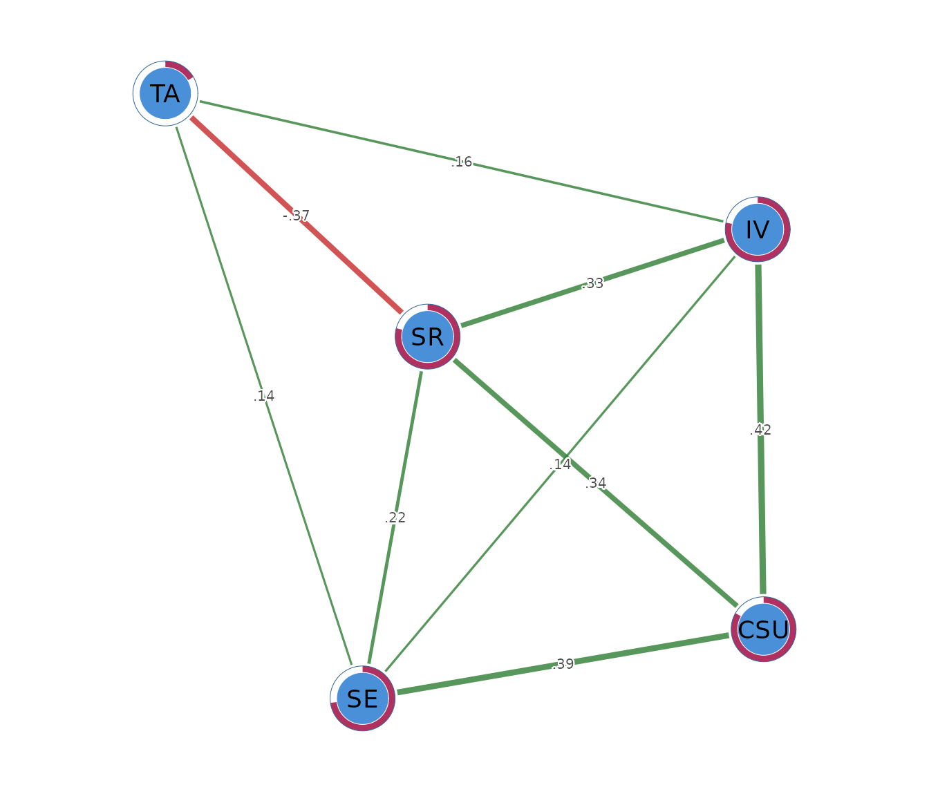

The figure summarizes the signs and relative magnitudes of the retained edges. Node placement comes from a layout algorithm and has no measurement scale. Interpretation should therefore use the printed edge and node tables as the primary numerical results.

Sensitivity to rank correlations

psychnet() accepts cor_method = "spearman" for a rank-based sensitivity analysis. This analysis asks whether the main structure persists when estimation depends on monotonic ranks and is less sensitive to extreme values.

spearman_net <- psychnet(data = SRL_GPT, method = "ggm", cor_method = "spearman")
spearman_net
#> <psychnet> ggm network
#>   nodes: 5   edges: 7   (undirected)
#>   optimality (KKT residual): 6.66e-16

summary(spearman_net)
#> <psychnet> ggm network
#>   nodes: 5   edges: 7   (undirected)
#>   optimality (KKT residual): 6.66e-16
#>   edge weight: range [-0.266, 0.483], mean 0.245

The Spearman model contains 7 edges, compared with 9 in the Pearson model. The positive CSU-IV, CSU-SE, CSU-SR, IV-SR, and SE-SR edges remain, as does the negative SR-TA edge. The IV-SE and SE-TA edges are removed. The main positive learning cluster and negative self-regulation to test-anxiety relation persist, while several weaker connections depend on the correlation estimator.

certificate(spearman_net)
#>   method  certificate kind certified
#> 1    ggm 6.661338e-16  kkt      TRUE

The Spearman fit has a residual of $1.55 \times 10^{-15}$ and is certified. Its numerical solution therefore satisfies the selected graph’s defining conditions to numerical precision.

Reporting the analysis

A report should state the variables, sample size, correlation estimator, missing-data procedure, selection criterion, value of $\gamma$, and whether the stepwise refinement was used. The edge table should be reported numerically. Interpretation should distinguish partial correlations from ordinary correlations and from causal effects.

The present analysis used Pearson correlations, ordinary BIC ($\gamma = 0$), and the default single-edge stepwise refinement on 300 complete observations. The selected network contained 9 edges. The largest positive edge was CSU-IV ($r = 0.422$), and the negative SR-TA edge was -0.370. The maximum-likelihood refit had a KKT residual of $1.33 \times 10^{-15}$. A Spearman sensitivity model retained the main pattern but selected 7 edges.

How stepwise selection works

The fitting procedure begins by generating candidate network structures across a graphical-lasso penalty path. At this stage, the path is a practical way to produce networks ranging from sparse to dense. Each distinct edge pattern is a candidate structure.

Every candidate structure is then refitted by unregularized maximum likelihood. The Bayesian information criterion scores the tradeoff between fit and the number of edges. The candidate with the smallest score becomes the starting network for a local stepwise refinement. The refinement tests single-edge additions and removals, retaining a change whenever it improves the criterion. It stops when no single-edge change improves the score.

The resulting graph is a local optimum among the one-edge alternatives examined by the search. A different correlation estimator or model-selection setting can lead to a different structure, as the Spearman analysis showed. The selected network should therefore be treated as an estimated model whose stability needs evaluation in a full study.

Mathematical foundations

This section states the model and selection criterion precisely. It can be skipped when the practical workflow is the main interest.

Gaussian graphical model

Let $\mathbf{X}$ follow a multivariate normal distribution with covariance matrix $\boldsymbol{\Sigma}$ and precision matrix $\mathbf{K} = \boldsymbol{\Sigma}^{-1}$. For $i \ne j$,

$$K_{ij} = 0 \quad \Longleftrightarrow \quad X_i \perp\!\!\!\perp X_j \mid \mathbf{X}_{\setminus\{i,j\}}.$$

The reported partial correlation is

$$\rho_{ij \cdot \mathrm{rest}} = -\frac{K_{ij}}{\sqrt{K_{ii}K_{jj}}}.$$

Information criterion

For a candidate graph with $E$ edges, sample size $n$, and $p$ nodes, the extended Bayesian information criterion is

$$\operatorname{EBIC}_{\gamma} = -2\ell(\widehat{\mathbf{K}}) + E\log(n) + 4E\gamma\log(p).$$

The default $\gamma = 0$ removes the final term and yields ordinary BIC. The selected graph is the candidate with the smallest criterion value, followed by the single-edge refinement.

Constrained maximum-likelihood certificate

Let $\mathbf{S}$ be the sample correlation matrix and $\mathbf{W} = \widehat{\mathbf{K}}^{-1}$ be the covariance matrix implied by the fitted precision matrix. For every retained edge and every diagonal entry, the constrained optimum satisfies the corresponding covariance equality between $\mathbf{W}$ and $\mathbf{S}$. Precision entries outside the selected graph are zero. certificate() reports the maximum absolute violation across these conditions. A value near machine precision indicates that the constrained fit satisfies them to numerical precision.

Predictability

For node $j$, the conditional residual variance is $1/K_{jj}$. Its explained variance is

$$R_j^2 = 1 - \frac{1}{K_{jj}S_{jj}},$$

where $S_{jj}$ is the marginal variance. net_predict() evaluates this identity for each node in the selected Gaussian graphical model.